

книги студ / color atlas of physiology 5th ed[1]. (a. despopoulos et al, thieme 2003)
.pdf13 Appendix
378
Since it is normally not possible to separately determine k and A of a biological membrane or cell layer, the product of the two (k · A) is often calculated as the ultrafiltration coefficient Kf
(m3 s–1 Pa–1) (cf. p. 152).
The transport of osmotically active particles causes water flow. Inversely, flowing water drags dissolved particles along with it. This type of solvent drag (! p. 24) is a form of convective transport.
Solvent drag does not occur if the cell wall is impermeable to the substance in question (σ = 1). Instead, the water will be retained on the side where the substance is located. In the case of the aforementioned epithelia, this means that the substances that cannot be reabsorbed from the tubule or intestinal lumen lead to osmotic diuresis (! p. 172) and diarrhea respectively. The latter is the mechanism of action of saline laxatives (! p. 262).
Oncotic Pressure / Colloid Osmotic Pressure
As all other particles dissolved in plasma, macromolecular proteins also exert an osmotic pressure referred to as oncotic pressure or colloid osmotic pressure. Considering its contribution of only 3.5 kPa (25 mm Hg) relative to the total osmotic pressure of the small molecular components of plasma, the oncotic pressure on a strictly semipermeable membrane could be defined as negligible. However, within the body, oncotic pressure is so important because the endothelium that lines the blood vessels allows small molecules to pass relatively easily (σ ! 0). According to equation 13.3, their osmotic pressure difference Δπ at the endothelium is virtually zero. Consequently, only the oncotic pressure difference of proteins is effective, as the endothelium is either partly or completely impermeable to them, depending on the capillary segment in question. Because the protein reflection coefficient σ #0 and the protein content of the plasma (ca. 75 g/L) are higher than that of the interstitium, these two factors counteract filtration, i.e., the blood pressure-driven outflow of plasma water from the endothelial lumen, making the endothelium an effective volume barrier between the plasma space and the interstitium.
If the blood pressure drives water out of the blood into the interstitium (filtration), the
plasma protein concentration and thus the oncotic pressure difference π will rise (! pp. 152, 208). This rise is much higher than equation 13.3 leads one to expect (! A). The difference is attributable to specific biophysical properties of plasma proteins. If there is a pres- sure-dependent efflux or influx of water out of or into the bloodstream, these relatively high changes in oncotic pressure difference automatically exert a counterpressure that limits the flow of water.
pH, pK, Buffers
The pH indicates the hydrogen ion [H+] concentration of a solution. According to Sörensen, the pH is the negative common logarithm of the molal H+ concentration in mol/kg H2O.
Examples:
1 mol/kg H2O = 100 mol/kg H2O = pH 0, 0.1 mol/kg H2O = 10–1 mol/kg H2O = pH 1, and so on up to 10-14 mol/kg H2O = pH 14.
Since glass electrodes are normally used to measure the pH, the H+ activity of the solution is actually being determined. Thus, the following rule applies:
pH = – log (fH · [H+]),
where fH is the activity coefficient of H+. Considering its ionic concentration (see above), the fH of plasma is !0.8.
The logarithmic nature of pH must be considered when observing pH changes. For example, a rise in pH from 7.4 (40 nmol/kg H2O) to pH 7.7 decreases the H+ activity by 20 nmol/ kg H2O, whereas an equivalent decrease (e.g., from pH 7.4 to pH 7.1) increases the H+ activity by 40 nmol/kg H2O.
The pK is fundamentally similar to the pH. It is the negative common logarithm of the dissociation constant of an acid (Ka) or of a base (Kb):
pKa = $log Ka
pKb = $log Kb.
For an acid and its corresponding base, pKa + pKb = 14, so that the value of pKa can be derived from that of pKb and vice versa.
The law of mass actions applies when a weak acid (AH) dissociates:
AH A– + H+ |
[13.5] |
It states that the product of the molal concentration (indicated by square brackets) of the dissociation products divided by the concentration of the nondissociated substance remains constant:
Despopoulos, Color Atlas of Physiology © 2003 Thieme
All rights reserved. Usage subject to terms and conditions of license.
H2O influx
Changes in oncotic
mL/100mL plasma
pressure of plasma proteins
+40 mmHg +30
+20
+10
Actual
No deviation
from
van’t Hoff ’s law
60 40 20
20 40 60 mL/100mL plasma
–10
H2O loss
–20
A. Physiological signification of deviations on oncotic pressure of plasma from van’t Hoff’s equation. A loss of water from plasma leads to a disproportionate rise in oncotic pressure, which counteracts the water loss. Conversely, the dilution of plasma due to the influx of water leads to a disproportionate drop in oncotic pressure, though less pronounced. Both of these are important mechanisms for maintaining a constant blood volume and preventing edema. (Adapted from Landis EM u. Pappenheimer JR. Handbook of Physiology. Section 2: Circulation, Vol. II. American Physiological Society: Washington D.C. 1963, S. 975.)
Dimensions and Units
Ka = |
[A–] · [H+] · fH |
[13.6] |
|
[AH] |
|||
|
|
Converted into logarithmic form (and inserting H+ activity for [H+]), the equation is transformed into:
log Ka = log |
[A–] |
+ log ([H+] · fH) |
[13.7] |
||
[AH] |
|||||
|
|
|
|
||
or |
|
|
|
|
|
$log ([H+] · fH) = $ log Ka + log |
[A–] |
[13.8] |
|||
[AH] |
|||||
|
|
|
|
||
Based on the above definitions for pH and pKa, it can also be converted into
pH = pKa + log |
[A–] |
[13.9] |
[AH] |
Because the concentration and not the activity of A– and AH is used here, pKa is concentration-dependent in nonideal solutions.
Equation 13.9 is the general form of the
Henderson–Hasselbalch equation (! p. 138ff.), which describes the relationship between the pH of a solution and the concentration ratio of a dissociated to an undissociated form of a solute. If [A–] = [AH], then the concentration ratio is 1/1 = 1, which corresponds to pH = pKa since the log of 1 = 0.
A weak acid (AH) and its dissociated salt (A–) form a buffer system for H+ and OH– ions:
Addition of H+ yields A– + H+ ! AH Addition of OH– yields AH + OH– ! A– + H2O. The buffering power of a buffer system is
greatest when [AH] = [A–], i.e., when the pH of the solution equals the pKa of the buffer.
Example: Both [A–] and [AH] = 10 mmol/L and pKa = 7.0. After addition of 2 mmol/L of H+ ions, the [A–]/ [AH] ratio changes from 10/10 to 8/12 since 2 mmol/
L of A– are consequently converted into 2 mmol/L of 379 AH. Since the log of 8/12 !-0.18, the pH decreases
Despopoulos, Color Atlas of Physiology © 2003 Thieme
All rights reserved. Usage subject to terms and conditions of license.
by 0.18 units to pH 6.82. If the initial [A–] /[AH] ratio had been 3/17, the pH would have dropped from an initial pH 6.25 (7 plus the log of 3/17 = 6.25) to pH 5.7 (7 + log of 1/19 = 5.7), i.e., by 0.55 pH units after addition of the same quantity of H+ ions.
|
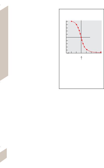
The titration of a buffer solution with H+ (or |
|
|
OH–) can be plotted to generate a buffering |
|
|
curve (! B). The steep part of the curve repre- |
|
|
sents the range of the best buffering power. |
|
|
The pKa value lies at the turning point in the |
|
|
middle of the steep portion of the curve. Sub- |
|
|
stances that gain (or lose) more than one H+ |
|
|
per molecule have more than one pK value and |
|
|
can therefore exert an optimal buffering action |
|
|
in several regions. Phosphoric acid (H3PO4) |
|
|
donates three H+ ions, thereby successively |
|
|
forming H2PO4–, HPO42–, and PO43–. The buffer |
|
Appendix |
pair HPO42–/H2PO4– with a pKa of 6.8 is impor- |
|
tant in human physiology (! p. 174ff.). |
||
|
||
|
The absolute slope, d[A–]/d(pH), of a buff- |
|
|
ering curve (plot of pH vs. [A–]) is a measure of |
|
13 |
buffering capacity (mol · L–1 · [ pH]–1; ! p. |
|
138). |
||
|
||
|
Powers and Logarithms |
|
|
Powers of ten are used to more easily and con- |
|
|
veniently write numbers that are much larger |
|
|
or smaller than 1. |
|
|
Examples: |
|
|
100 = 10 · 10 = 102 |
|
|
1000 = 10 · 10 · 10 = 103 |
|
|
10 000 = 10 · 10 · 10 · 10 = 104, etc. |
|
|
In this case, the exponent denotes the |
|
|
amount of times ten is multiplied by itself. If |
|
|
the number is not an exact power of ten (e.g., |
|
|
34 500), divide it by the next lowest decimal |
|
|
power (10 000) and use the quotient (3.45) as a |
|
|
multiplier to express the result as 3.45 · 104. |
|
|
The number 10 can also be expressed ex- |
|
|
ponentially (101). Numbers much smaller than |
|
|
1 are annotated using negative exponents. |
|
|
Examples: |
|
|
1 = 10 %10 = 100 |
|
|
0.1 = 10 %10 %10 = 10–1 |
|
|
0.01 = 10 %10 %10 = 10-2, etc. |
|
|
Similar to the large numbers above, num- |
|
|
bers that are not exact powers of ten are ex- |
|
|
pressed using multipliers, e.g., |
|
|
0.04 = 4 · 0.01 = 4 · 10-2. |
|
380 |
Note: When writing numbers smaller than |
|
|
1, the (negative) exponent corresponds to the |
Concentration ratio of buffer pair [AH]:[A–]
10:0 9:1
8:2 7:3 6:4 5:5 4:6
3:7 2:8 1:9
0:10 |
3 |
4 |
5 |
6 |
7 |
8 |
9 |
|
pH
(pH=pK)
B. Buffering Curve. Graphic representation of the relationship between pH and the concentration ratio of buffer acid/buffer base [AH]/[A–] as a function of pH. The numerical values are roughly equivalent to those of the buffer pair acetic acid/ acetate (pKa = 4.7). The buffering power of a buffer system is greatest when [AH] = [A–], i.e., when the pH of the solution equals the pKa of the buffer (broken lines).
position of the 1 after the decimal point; therefore, 0.001 = 10-3. When writing numbers greater than 10, the exponent corresponds to the number of decimal positions to the left of the decimal point minus 1; therefore, 1124.5 = 1.245 · 103.
Exponents can also be used to represent units of measure, e.g., m3. As in the case of 103, the base element (meters) is multiplied by itself three times (m · m · m; ! p. 372). Negative exponents are also used to express units of measure. As with 1/10 = 10–1, 1/s can be written as s–1, mol/L as mol · L–1, etc.
There are specific rules for performing calculations with powers of ten. Addition and subtraction are possible only if the exponents are identical, e.g.,
(2.5 · 102) + (1.5 · 102) = 4 · 102.
Unequal exponents, e.g., (2 · 103) + (3 · 102), must first be equalized:
(2 · 103) + (0.3 · 103) = 2.3 · 103.
Despopoulos, Color Atlas of Physiology © 2003 Thieme
All rights reserved. Usage subject to terms and conditions of license.
The exponents of the multiplicands are added together when multiplying powers of 10, and the denominator is subtracted from the numerator when dividing powers of ten.
Examples:
102 · 103 = 102+ 3 = 105 104 %102 = 104 - 2 = 102 102 %104 = 102 - 4 = 10-2
The usual mathematical rules apply to the multipliers of powers of ten, e.g.,
(3 · 102 · (2 · 103) = (2 · 3) · (102+ 3) = 6 · 105. Logarithms. There are two kinds of loga-
rithms: common and natural. Logarithmic calculations are performed using exponents alone. The common (decimal) logarithm (log or lg) is the power or exponent to which 10 must be raised to equal the number in question. The common logarithm of 100 (log 100) is 2, for example, because 102 = 100. Decimal logarithms are commonly used in physiology, e.g., to define pH values (see above) and to plot the pressure of sound on a decibel scale (!p. 363).
Natural logarithms (ln) have a natural base of 2.71828..., also called base e. The common logarithm (log x) equals the natural logarithm of x (ln x) divided by the natural logarithm of 10 (ln 10), where ln 10 = 2.302585. The following rules apply when converting between natural and common logarithms:
log x = (ln x)/2.3 ln x = 2.3 · log x.
When performing mathematical operations with logarithms, the type of operation is reduced by one rank—multiplication becomes addition, potentiation becomes multiplication, and so on.
Examples:
log (a · b) = log a + log b log (a/b) = log a - log b log an = n · log a
log n!"a = (log a)/n
Special cases: log 10 = ln e = 1 log 1 = ln 1 = 0 log 0 = ln 0 = & '
Graphic Representation of Data
Graphic plots of data are used to provide a |
|
||||||||
clear and concise representation of measure- |
|
||||||||
ments, e.g., body temperature over the time of |
|
||||||||
day (! C). The axes on which the measure- |
Data |
||||||||
ments (e.g., temperature and time) are plotted |
|||||||||
|
|||||||||
are called coordinates. The vertical axis is re- |
of |
||||||||
ferred to as the ordinate (temperature) and the |
|||||||||
Representation |
|||||||||
horizontal axis is the abscissa (time). It is cus- |
|||||||||
|
|||||||||
tomary to plot the first variable x (time) on the |
|
||||||||
abscissa and the other dependent variable y |
|
||||||||
(temperature) on the ordinate. The abscissa is |
|
||||||||
therefore called the x-axis and the ordinate the |
|
||||||||
y-axis. This method of graphically plotting data |
Graphic |
||||||||
can be used to illustrate the connection be- |
|||||||||
tween any two related dimensions imaginable, |
|||||||||
e.g., to describe the relationship between |
|||||||||
height and age, lung capacity and intrapulmo- |
Logarithms, |
||||||||
other. For example, the plot of height (ordi- |
|||||||||
nary pressure, etc. (!p. 117). |
|
|
|
|
|
||||
Plotting of data makes it easier to determine |
|
||||||||
whether two variables correlate with each |
|
||||||||
nate) over age (abscissa) shows that the height |
|
||||||||
increases during the growth years and reaches |
|
||||||||
a plateau at the age of about 17 years. This |
|
||||||||
means that height is related to age in the first |
|
||||||||
phase of life, but is largely independent of age |
|
||||||||
in the second phase. A correlation does not |
|
||||||||
necessarily indicate a causal relationship. A |
|
||||||||
decrease in the birth rate in Alsace-Lorraine, |
|
||||||||
for example, correlated with a decrease in the |
|
||||||||
number or nesting storks for a while. |
|
|
|
|
|||||
When plotting variables of wide-ranging di- |
|
||||||||
mensions (e.g., 1 to 100 000) on a coordinate |
|
||||||||
|
|
|
|
|
|
|
|
|
|
37.5 |
|
|
|
|
|
|
|
|
|
|
|
|
|
|
|
|
|
||
°C |
|
|
|
|
|
|
|
|
|
temperatureBody (rectal,at rest) |
|
|
|
|
|
|
|
|
|
37.0 |
|
|
|
|
|
|
|
|
|
36.5 |
|
|
|
|
|
|
|
|
|
12 |
6 |
12 |
6 |
12 |
|
|
|||
|
|
|
|||||||
|
p.m. p.m. |
a.m. a.m. p.m. |
|
||||||
|
|
Time of day |
|
|
|
|
|
||
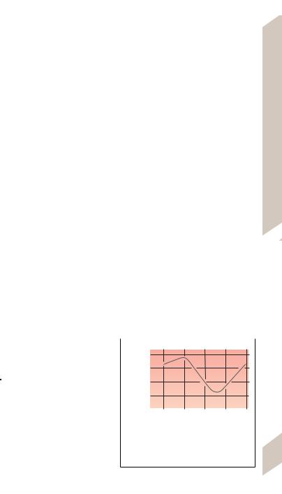
C. Illustration of how to plot data on a coordinate system. The plot in this example shows the
relationship between body temperature (rectal, 381 at rest) and time of day.
Despopoulos, Color Atlas of Physiology © 2003 Thieme
All rights reserved. Usage subject to terms and conditions of license.

13 Appendix
2y
ln |
|
|
|
|
|
|
|
|
|
|
||
|
|
|
|
|
|
|
|
|
|
|
|
|
|
|
|
|
y |
|
|
3 |
|
|
|
|
|
|
|
|
|
ln |
|
|
|
|
|
|
|
|
|
y=a·eb·x |
|
|
|
|
|
|
|
|
|
|
|
|
|
|
|
|
|
|
|
|
|
|
|
|
|
lny=lna + b!x |
|
|
|
|
|
|
y=a·xb |
||||
|
|
|
|
|
|
|
|
|||||
|
|
|
|
|
|
|
|
|
|
|
|
|
|
|
|
|
|
|
|
|
lny=lna + b!lnx |
|
|
|
|
|
Exponential function |
|
|
|
|
|
|
|
|
|
|
|
|
|
|
|
|
|
|
|
|
|
|
||
|
|
|
|
|
|
|
|
|
|
|
|
|
|
x (linear) |
Power |
function |
|||||||||
|
|
|
||||||||||
1 |
|
|
|
|
|
|
|
|
|
|
|
|
|
|
|
|
|
|
|
|
|
ln x |
|||
y(linear) |
|
|
(linear) |
|
|
|
||||||
|
|
4 |
|
|
|
|
|
|||||
|
|
|
|
|
|
|
|
|
|
|
|
|
|
|
|
|
|
y |
|
|
|
|
|
|
|
|
Linear function |
|
|
|
|
|
|
|
||||
|
|
|
|
|
|
y=a + b!lnx |
|
|
||||
|
|
|
|
|
|
|
|
|
|
|||
|
|
|
|
|
|
Logarithmic function |
||||||
x (linear)
ln x
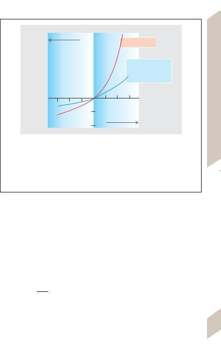
D. Types of functions. D1: Linear function (violet), exponential function (red), logarithmic function (blue), and power function (green) showing linear plotting of data on both axes. The three curves can be made into a straight line (linearized) by logarithmically plotting the data on the y-axis (D2: exponential function) or on the x-axis (D4: logarithmic function) or both (D3: power function).
system, it can be impossible to plot small values individually without having the axes become extremely long. This problem can be solved by plotting the data as powers of 10 or logarithms. For example, 1, 10, 100, and 1000
382are written as 100, 101, 102, and 103 or as logarithms 0, 1, 2, and 3. This makes it possible to
obtain a relatively accurate graphic representation of very small numbers, and all the numbers fit on an axis of reasonable length (cf. sound curves on p. 363 B).
Correlations can be either linear or nonlinear. Linear correlations (! D1, violet line) obey the linear relationship
Despopoulos, Color Atlas of Physiology © 2003 Thieme
All rights reserved. Usage subject to terms and conditions of license.
y = ax + b,
where a is the slope of the line and b is the point, or intercept (at x = 0), where it intersects the y-axis.
Many correlations are nonlinear. For simpler functions, graphic linearization can be achieved via a nonlinear (logarithmic) plot of the x and/or y values. This allows for the extrapolation of values beyond the range of measurement (see below) or for the generation of calibration curves from only two points. In addition, this method also permits the calculation of the “mean” correlation of scattered x-y pairs using regression lines.
An exponential function (! D1, red curve), such as
y = a · eb · x,
can be linearized by plotting ln y on the y-axis (!D2):
ln y = ln a + b · x,
where b is the slope and ln a is the intercept. A logarithmic function (! D1, blue curve),
such as
y = a + b · ln x,
can be linearized by plotting ln x on the x-axis (! D4), where b is the slope and a is the intercept.
A power function (! D1, green curve), such
as
y = a · xb,
can be graphically linearized by plotting ln y and ln x on the coordinate axes (! D3) because
ln y = ln a + b · ln x,
where b is the slope and ln a is the intercept.
Note: The condition x or y = 0 does not exist on logarithmic coordinates because ln 0 = '. Nevertheless, ln a is still called the intercept in the equation when the logarithmic abscissa (! D3,4) is intercepted by the ordinate at ln x = 0, i.e., x = 1.
Instead of plotting ln x and/or ln y on the x- and/or y-axis, they can be plotted on logarithmic paper on which the ordinate or abscissa (semi-log paper) or both coordinates (log-log paper) are plotted in logarithmic units. In such cases, a is no longer treated as the intersect because the position of a depends on site of intersection of the x-axis by the y-axis. All values (0 are possible.
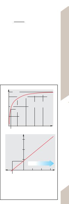
Other nonlinear functions can also be graphically linearized using an appropriate plotting method. Take, for example, the Michaelis– Menten equation (! E1), which applies to
many enzyme reactions and carrier-mediated transport processes:
J = Jmax · |
C |
[13.10] |
KM + C |
where J is the actual rate of transport (e.g., in
mol · m–2 · s–1), Jmax is the maximal transport rate, C (mol · m–3) is the actual concentration of
the substance to be transported, and KM is the concentration (half-saturation concentration)
at 1/2 Jmax.
One of the three commonly used linear rearrangements of the Michaelis–Menten equation, the Lineweaver–Burk plot, states:
1/J = (KM/Jmax) · (1/C) + 1/Jmax, |
[13.11] |
Consequently, a plot of 1/J on the y-axis and 1/C on the x-axis results in a straight line (! E2). While a plot of J over C (! E1) does not
1 |
|
Jmax |
|
J |
|
|
|
J = Jmax !C/(KM+C)
1/2Jmax
|
0 |
C |
|
KM |
|
2 |
1/J |
|
|
|
|
|
1/Jmax |
Range of |
|
|
|
|
|
measurement |
|
0 |
1/C |
|
–1/KM |
|
E. Two methods of representing the Mi- chaelis–Menten equation: The data can be plotted as a curve of J over C (E1), or as 1/J over 1/C in linearized form (E2). In the latter case, Jmax and KM are determined by extrapolating the data outside the range of measurement.
Graphic Representation of Data
383
Despopoulos, Color Atlas of Physiology © 2003 Thieme
All rights reserved. Usage subject to terms and conditions of license.

13 Appendix
permit accurate extrapolation of Jmax (because an infinitely high concentration of C would be required), the linear rearrangement (! E2) makes it possible to generate a regression line that can be extrapolated to C = ' from the measured data. Since 1/C is equal to 1/' = 0,1/Jmax lies on the y-axis at x = 0 (! E2). The reciprocal of this value is Jmax. Insertion of 1/J = 0 into equation 13.11 yields
0 = (KM/Jmax) · (1/C) + 1/Jmax |
[13.12] |
or 1/KM = $1/C, so that KM can be derived from the negative reciprocal of the x-axis intersect, which corresponds to 1/J = 0 (! E2).
Reference Values in Physiology
|
The Greek Alphabet |
|
|
|
|
|
|
|
α |
Α |
alpha |
( |
Β |
beta |
|
γ |
* |
gamma |
|
δ |
|
delta |
|
ε |
Ε |
epsilon |
|
. |
/ |
zeta |
|
η |
Η |
eta |
|
), θ |
Θ |
theta |
|
ι |
Ι |
iota |
|
κ |
Κ |
kappa |
|
λ |
Λ |
lamda |
|
µ |
Μ |
mu |
|
ν |
Ν |
nu |
|
= |
> |
xi |
|
? |
@ |
omicron |
|
π |
Π |
pi |
|
* |
Ρ |
rho |
|
σ, C |
Σ |
sigma |
|
τ |
Τ |
tau |
|
υ |
Υ |
upsilon |
|
φ |
Φ |
phi |
|
K |
L |
chi |
|
ψ |
Ψ |
psi |
|
ω |
Ω |
omega |
|
|
|
|
|
Total body and cells
Chemical composition of 1 kg fat-free body mass of an adult
Distribution of water in adult (child) as percentage of body weight (cf. p. 168)
Ion concentrations in ICF and ECF
720 g water, 210 g protein, 22.4 g Ca, 12 g P, 2.7 g K, 1.8 g Na, 1.8 g Cl, 0.47 g Mg
Intracellular: 40% (40%); interstitium: 15% (25%); plasma: 5% (5%)
See p. 93 C
Cardiovascular system
|
Weight of heart |
250–350 g |
|
Cardiac output at rest (maximal) |
5–6 L/min (25 L/min); cf. p. 186 |
|
Resting pulse = sinus rhythm |
60–75 min-1 or bpm |
|
AV rhythm |
40–55 min-1 |
|
Ventricular rhythm |
25–40 min-1 |
|
Arterial blood pressure (Riva–Rocci) |
120/80 mm Hg (16/10.7 kPa) systolic/diastolic |
|
Pulmonary artery pressure |
20/7 mm Hg (2.7/0.9 kPa) systolic/diastolic |
|
Central venous pressure |
3–6 mm Hg (0.4–0.8 kPa) |
|
Portal venous pressure |
3–6 mm Hg (0.4–0.8 kPa) |
|
Ventricular volume at end of diastole/systole |
120 mL/40 mL |
|
Ejection fraction |
0.67 |
|
Pressure pulse wave velocity |
Aorta: 3–5 m/s; arteries: 5–10 m/s; |
|
|
veins: 1–2 m/s |
384 |
Mean velocity of blood flow |
Aorta: 0.18 m/s; capillaries: 0.0002–0.001 m/s; |
|
|
venae cavae: 0.06 m/s |
Despopoulos, Color Atlas of Physiology © 2003 Thieme
All rights reserved. Usage subject to terms and conditions of license.

Blood flow in organs at rest |
|
|
|
(See also pp. 187 A, 213 A) |
% of cardiac output |
per gram of tissue |
|
Heart |
4% |
0.8 mL/min |
|
Brain |
13% |
0.5 mL/min |
|
Kidneys |
20% |
4 mL/min |
|
GI tract (drained by portal venous system) |
16% |
0.7 mL/min |
|
Liver (blood supplied by hepatic artery) |
8% |
0.3 mL/min |
|
Skeletal muscle |
21% |
0.04 mL/min |
|
Skin and miscellaneous organs |
18% |
— |
|
|
|
|
|
Lungs and gas transport |
Men |
Women |
|
Total lung capacity (TLC) |
7 L |
6.2 L |
|
Vital capacity (VC); cf. p. 112 |
5.6 L |
5 L |
|
Tidal volume (VT) at rest |
0.6 L |
0.5 L |
|
Inspiratory reserve volume |
3.2 L |
2.9 L |
|
Expiratory reserve volume |
1.8 L |
1.6 L |
|
Residual volume |
1.4 L |
1.2 L |
|
Max. breathing capacity in 30 breaths/min |
110 L |
100 L |
|
Partial pressure of O2 |
Air: 21.17 kPa |
(159 mm Hg) |
|
|
Alveolar: 13.33 kPa |
(100 mm Hg) |
|
|
Arterial: 12.66 kPa |
(95 mm Hg) |
|
|
Venous 5.33 kPa |
(40 mm Hg) |
|
Partial pressure of CO2 |
Air: 0.03 kPa |
(0.23 mm Hg) |
|
|
Alveolar: 5.2 kPa |
(39 mm Hg) |
|
|
Arterial: 5.3 kPa |
(40 mm Hg) |
|
|
Venous: 6.1 kPa |
(46 mm Hg) |
|
Respiratory rate (at rest) |
16 breaths/min |
|
|
Dead space volume |
150 mL |
|
|
Oxygen capacity of blood |
180–200 mL O2/L blood = 8–9 mmol O2/L blood |
||
Respiratory quotient |
0.84 (0.7–1.0) |
|
|
|
|
|
|
Kidney and excretion |
|
|
|
Renal plasma flow (RPF) |
480–800 mL/min per 1.73 m2 body surface |
||
|
area |
|
|
Glomerular filtration rate (GFR) |
80–140 mL/min per 1.73 m2 body surface area |
||
Filtration fraction (GFR/RPF) |
0.19 |
|
|
Urinary output |
0.7–1.8 L/day |
|
|
Osmolality of urine |
250–1000 mOsm/kg H2O |
||
Na+ excretion |
50–250 mmol/day |
|
|
K+ excretion |
25–115 mmol/day |
|
|
Glucose excretion |
"300 mg/day = 1.67 mmol/day |
||
Nitrogen excretion |
150–250 mg/kg/day |
|
|
Protein excretion |
10–200 mg/day |
|
|
Urine pH |
4.5–8.2 |
|
|
Titratable acidity |
10–30 mmol/day |
|
|
Urea excretion |
10–20 g/day = 166–333 mmol/day |
||
Uric acid excretion |
300–800 mg/day = 1.78–6.53 mmol/day |
||
Creatinine excretion |
0.56–2.1 g/day = 4.95–18.6 µg/day |
||
Despopoulos, Color Atlas of Physiology © 2003 Thieme
All rights reserved. Usage subject to terms and conditions of license.
Reference Values in Physiology
385

13 Appendix
Nutrition and metabolism |
Men |
Women |
Energy expenditure during various activities |
|
|
! Bed rest |
6500 kJ/d |
5400 kJ/d |
|
(1550 kcal/d) |
(1300 kcal/d) |
! Light office work |
10 800 kJ/d |
9600 kJ/d |
|
(2600 kcal/d) |
(2300 kcal/d) |
! Walking (4.9 km/h) |
3.3 kW |
2.7 kW |
! Sports (dancing, horseback riding, swimming) |
4.5–6.8 kW |
3.6–5.4 kW |
Functional protein minimum |
1 g/kg body weight |
|
Vitamins, optimal daily intake |
A: 10 000–50 000 IU; D: 400–600 IU |
|
(IU = international units) |
E: 200–800 IU; K: 65–80 µg; B1, B2, B5, B6: |
|
|
25–300 mg of each; B12: 25–300 µg; folate: |
|
|
0.4–1.2 mg; H: 25–300 µg; C: 500–5000 mg |
|
Electrolytes and trace elements, |
Ca: 1–1.5 g; Cr: 200–600 µg; Cu: 0.5–2 mg; |
|
optimal daily intake |
Fe: 15–30 mg: I: 50–300 µg; K+: 0.8–1.5 g; |
|
|
Mg: 500–750 mg; Mn: 15–30 mg; |
|
|
Mo: 45–500 µg; Na+: 2 g; P: 200–400 mg; |
|
|
Se: 50–400 µg; Zn: 22–50 mg |
|
|
|
|
Nervous Systems, muscles |
|
|
Duration of an action potential |
Nerve: 1–2 ms; skeletal muscle: 10 ms; |
|
|
myocardium: 200 ms |
|
Nerve conduction rate |
See p. 49 C |
|
|
Blood and other bodily fluids |
(see also Tables 9.1, and 9.2 on pp. 186, 187) |
|
|
Blood (in adults) |
Men: |
Women: |
|
Blood volume (also refer to table on p. 88) |
4500 mL |
3600 mL |
|
Hematocrit |
0.40–0.54 |
0.37–0.47 |
|
Red cell count (RBC) |
4.5–5.9 · 1012/L |
4.2–5.4 · 1012/L |
|
Hemoglobin (Hb) in whole blood |
140–180 g/L |
120–160 g/L |
|
|
(2.2–2.8 mmol/L) |
(1.9–2.5 mmol/L) |
|
Mean corpuscular volume (MCV) |
80–100 fL |
|
|
Mean corpuscular Hb concentration (MCHC) |
320–360 g/L |
|
|
Mean Hb concentration in single RBC (MCH) |
27–32 pg |
|
|
Mean RBC diameter |
7.2–7.8 µm |
|
|
Reticulocytes |
0.4–2% (20–75 · 109/L) |
|
|
Leukocytes (also refer to table on p. 88) |
3–11 · 109/L |
|
|
Platelets |
170–360 · 109/L |
180–400 · 109/L |
|
Erythrocyte sedimentation rate (ESR) |
"10 mm in first hour "20 mm in first hour |
|
|
Proteins |
|
|
|
Total |
66–85 g/L serum |
|
|
Albumin |
35–50 g/L serum |
55–64 % of total |
|
α1-globulins |
1.3–4 g/L serum |
2.5–4 % of total |
|
α2-globulins |
4–9 g/L serum |
7–10% of total |
|
(-globulins |
6–11 g/L serum |
8–12% of total |
|
γ-globulins |
13–17 g/L serum |
12–20% of total |
|
Coagulation |
(See p. 102 for coagulation factors) |
|
|
Thromboplastin time (Quick) |
0.9–1.15 INR (international normalized ratio) |
|
386 |
Partial thromboplastin time |
26–42 s |
|
|
Bleeding time |
"6 min |
|
Despopoulos, Color Atlas of Physiology © 2003 Thieme
All rights reserved. Usage subject to terms and conditions of license.

Parameters of glucose metabolism |
|
|
Glucose concentration in venous blood |
3.9–5.5 mmol/L |
(70–100 mg/dL) |
Glucose concentration in capillary blood |
4.4–6.1 mmol/L |
(80–110 mg/dL) |
Glucose concentration in plasma |
4.2–6.4 mmol/L |
(75–115 mg/dL) |
Limit for diabetes mellitus in plasma |
(7.8 mmol/L |
((140 mg/dL) |
HBA1c (glycosylated hemoglobin A) |
3.2–5.2% |
|
Parameters of lipid metabolism |
|
|
Triglycerides in serum |
"1.71 mmol/L |
("150 mg/dL) |
Total cholesterol in serum |
"5.2 mmol/L |
("200 mg/dL) |
HDL cholesterol in serum |
(1.04 mmol/L |
((40 mg/dL) |
Substances excreted in urine |
|
|
Urea concentration in serum |
3.3–8.3 mmol/L |
(20–50 mg/dL) |
Uric acid concentration in serum |
150–390 µmol/L |
(2.6–6.5 mg/dL) |
Creatinine concentration in serum |
36–106 µmol/L |
(0.4–1.2 mg/dL) |
Bilirubin |
|
|
Total bilirubin in serum |
3.4–17 µmol/L |
(0.2–1 mg/dL) |
Direct bilirubin in serum |
0.8–5.1 µmol/L |
(0.05–0.3 mg/dL) |
Electrolytes and blood gases |
|
|
Osmolality |
280–300 mmol/kg H2O |
|
Cations in serum: |
Na+ |
135–145 mmol/L |
|
K+ |
3.5–5.5 mmol/L |
|
Ionized Ca2+ |
1.0–1.3 mmol/L |
|
Ionized Mg2+ |
0.5–0.7 mmol/L |
Anions in serum: |
Cl- |
95–108 mmol/L |
|
H2PO4- + HPO42- |
0.8–1.5 mmol/L |
pH |
|
7.35–7.45 |
Standard bicarbonate |
|
22–26 mmol/L |
TotaL buffer bases |
|
48 mmol/L |
Oxygen saturation |
|
96% arterial; 65–75% |
|
|
mixed venous |
Partial pressure of O2 at half saturation (P0.5) |
|
3.6 kPa (27 mmHg) |
|
|
|
Cerebrospinal fluid |
|
|
Pressure in relaxed horizontal position |
1.4 kPa (10.5 mmHg) |
|
Specific weight |
1.006–1.008 g/L |
|
Osmolality |
290 mOsm/kg H2O |
|
Glucose concentration |
45–70 mg/dL (2.5–3.9 mmol/L) |
|
Protein concentration |
0.15–0.45 g/L |
|
IgG concentration |
"84 mg/dL |
|
White cell count |
"5 WBC/ µL |
|
|
|
|
Reference Values in Physiology
387
Despopoulos, Color Atlas of Physiology © 2003 Thieme
All rights reserved. Usage subject to terms and conditions of license.