

1manly_b_f_j_statistics_for_environmental_science_and_managem
.pdf56Statistics for Environmental Science and Management, Second Edition
3.Identify inputs to the decision: Determine the data needed to answer the important questions
4.Define the study boundaries: Specify the time periods and spatial areas to which decisions will apply; determine when and where to gather data
5.Develop the analytical approach: Define the parameter of interest, specify action limits, and integrate the previous DQO outputs into a single statement that describes the logical basis for choosing among possible alternative actions
6.Specify performance or acceptance criteria: Specify tolerable decision error probabilities (probabilities of making the wrong decisions) based on the consequences of incorrect decisions
7.Develop the plan for obtaining data: Consider alternative sampling designs, and choose the one that meets all the DQOs with the minimum use of resources
The output from each step influences the choices made later, but it is important to realize that the process is iterative, and the carrying out of one step may make it necessary to reconsider one or more earlier steps. Steps 1–6 should produce the Data Quality Objectives that are needed to develop the sampling design at step 7.
Preferably, a DQO planning team usually consists of technical experts, senior managers, a statistical expert, and a quality assurance/quality control (QA/QC) advisor. The final product is a data-collection design that meets the qualitative and quantitative needs of the study, and much of the information generated during the process is used for the development of quality assurance project plans (QAPPs) and the implementation of the data quality assessment (DQA) process. These are all part of the US EPA’s system for maintaining quality in its operations. More information about the DQO process, with reference documents, can be obtained from the EPA’s guidance document (US EPA 2006).
2.16 Chapter Summary
•A crucial early task in any sampling study is to define the population of interest and the sample units that make up this population. This may or may not be straightforward.
•Simple random sampling involves choosing sample units in such a way that each unit is equally likely to be selected. It can be carried out with or without replacement.
•Equations for estimating a population mean, total, and proportion are provided for simple random sampling.
Environmental Sampling |
57 |
•Sampling errors are those due to the random selection of sample units for measurement. Nonsampling errors are those from all other sources. The control of both sampling and nonsampling errors is important for all studies, using appropriate protocols and procedures for establishing data quality objectives (DQO) and quality control and assurance (QC/QA).
•Stratified random sampling is sometimes useful for ensuring that the units that are measured are well representative of the population. However, there are potential problems due to the use of incorrect criteria for stratification or the wish to use a different form of stratification to analyze the data after they have been collected.
•Equations for estimating the population mean and total are provided for stratified sampling.
•Post-stratification can be used to analyze the results from simple random sampling as if they had been obtained from stratified random sampling.
•With systematic sampling, the units measured consist of every kth item in a list, or are regularly spaced over the study area. Units may be easier to select than they are with random sampling, and estimates may be more precise than they would otherwise be because they represent the whole population well. Treating a systematic sample as a simple random sample may overestimate the true level of sampling error. Two alternatives to this approach (imposing a stratification and joining sample points with a serpentine line) are described.
•Cluster sampling (selecting groups of close sample units for measurement) may be a cost-effective alternative to simple random sampling.
•Multistage sampling involves randomly sampling large primary units, randomly sampling some smaller units from each selected primary unit, and possibly randomly sampling even smaller units from each secondary unit, etc. This type of sampling plan may be useful when a hierarchical structure already exists in a population.
•Composite sampling is potentially valuable when the cost of measuring sample units is much greater than the cost of selecting and collecting them. It involves mixing several sample units from the same location and then measuring the mixture. If there is a need to identify sample units with extreme values, then special methods are available for doing this without measuring every sample unit.
•Ranked-set sampling involves taking a sample of m units and putting them in order from the smallest to largest. The largest unit only is then measured. A second sample of m units is then selected, and the second largest unit is measured. This is continued until the mth sample of m units is taken and the smallest unit is measured. The mean of the m measured units will then usually be a more accurate

58 Statistics for Environmental Science and Management, Second Edition
estimate of the population mean than the mean of a simple random sample of m units.
•Ratio estimation can be used to estimate a population mean and total for a variable X when the population mean is known for a second variable U that is approximately proportional to X. Regression estimation can be used instead if X is approximately linearly related to U.
•Double sampling is an alternative to ratio or regression estimation that can be used if the population mean of U is not known, but measuring U on sample units is inexpensive. A large sample is used to estimate the population mean of U, and a smaller sample is used to estimate either a ratio or linear relationship between X and U.
•Methods for choosing sample sizes are discussed. Equations are provided for estimating population means, proportions, differences between means, and differences between proportions.
•Unequal-probability sampling is briefly discussed, where the sampling process is such that different units in a population have different probabilities of being included in a sample. Horvitz-Thompson estimators of the total population size and the total for a variable Y are stated.
•The U.S. EPA Data Quality Objective (DQO) process is described. This is a formal seven-step mechanism for ensuring that sufficient data are collected to make required decisions with a reasonable probability that these are correct, and that only the minimum amount of necessary data are collected.
Exercises
Exercise 2.1
In a certain region of a country there are about 200 small lakes. A random sample of 25 of these lakes was taken, and the sulfate levels (SO4, mg/L) were measured, with the following results:
6.5 |
5.5 |
4.8 |
7.4 |
3.7 |
7.6 |
1.6 |
1.5 |
1.4 |
4.6 |
7.5 |
5.8 |
1.5 |
3.8 |
3.9 |
1.9 |
2.4 |
2.7 |
3.2 |
5.2 |
2.5 |
1.4 |
3.5 |
3.8 |
5.1 |
|
|
|
|
|
1.Find an approximate 95% confidence interval for the mean sulfate level in all 200 lakes.
2.Find an approximate 95% confidence interval for the percentage of lakes with a sulfate level of 5.0 or more.
Environmental Sampling |
59 |
Exercise 2.2
Given the data from question 2.1, suppose that you have to propose a sampling design to estimate the difference between the SO4 levels in two different regions of the same country, both containing approximately 200 small lakes. What sample sizes do you propose to obtain confidence limits of about x1 − x2 ± 0.75?
Exercise 2.3
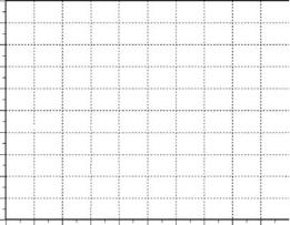
A study involved taking 40 partly systematic samples from a 1 × 1-m grid in a 1-ha field and measuring the sand content (%) of the soil. The measurements on sand content are as shown in Figure 2.9.
1.Estimate the mean sand content of the field with a standard error and 95% confidence limits, treating the sample as being effectively a random sample of points.
2.Estimate the mean sand content of the field with a standard error and 95% confidence limits using the first of the US EPA methods described in Section 2.9 (combining adjacent points into strata and using the stratified sampling formulae).
3.Estimate the mean sand content in the field, with a standard error and 95% confidence limits, using the second method recommended by the US EPA (joining points with a serpentine line).
4.Compare the results found in items 1 to 3 above and discuss reasons for the differences, if any.
Y
Figure 2.9
Sand content (%)
100 |
|
|
|
|
|
|
|
|
|
|
|
|
|
|
90 |
|
|
56.0 |
57.3 |
|
|
56.0 |
57.3 |
|
|||||
80 |
|
|
|
|
|
|
58.1 |
|
||||||
54.7 |
56.6 |
|
|
|
57.0 |
57.8 |
|
|
|
|||||
70 |
53.7 |
|
|
|
|
|||||||||
|
|
|
|
|
|
|||||||||
57.2 |
|
55.5 |
|
57.8 |
|
|||||||||
60 |
|
|
55.5 |
|
|
53.8 |
|
|
|
|||||
|
|
|
|
|
|
|
|
|
||||||
50 |
|
|
|
57.5 |
|
|
|
59.9 |
|
|
||||
|
|
|
52.6 |
|
58.4 |
|
|
|||||||
40 |
|
57.3 |
|
|
|
56.1 |
|
60.1 |
|
|
||||
30 |
|
51.7 |
|
|
|
|
|
|
61.9 |
|
||||
|
|
|
54.4 |
|
|
58.7 |
|
|
|
|||||
|
|
|
|
|
|
|
|
|
|
|
||||
20 |
55.9 |
|
59.5 |
54.4 |
|
58.5 |
62.1 |
|
|
|||||
10 |
|
|
64.9 |
|
61.2 |
58.4 |
|
|
|
|||||
56.5 |
|
57.0 |
|
|
63.5 |
59.8 |
|
|||||||
0 |
58.8 |
|
|
|
63.8 |
|
|
|||||||
0 |
10 |
20 |
30 |
40 |
50 |
60 |
70 |
80 |
90 |
100 |
||||
|
||||||||||||||
X
from soil samples taken at different locations in a field.

3
Models for Data
3.1 Statistical Models
Many statistical analyses are based on a specific model for a set of data, where this consists of one or more equations that describe the observations in terms of parameters of distributions and random variables. For example, a simple model for the measurement X made by an instrument might be
X = θ + ε
where θ is the true value of what is being measured, and ε is a measurement error that is equally likely to be anywhere in the range from −0.05 to +0.05.
In situations where a model is used, an important task for the data analyst is to select a plausible model and to check, as far as possible, that the data are in agreement with this model. This includes examining both the form of the equation assumed and the distribution or distributions that are assumed for the random variables.
To aid in this type of modeling process there are many standard distributions available, the most important of which are considered in the following two sections of this chapter. In addition, there are some standard types of models that are useful for many sets of data. These are considered in the later sections of this chapter.
3.2 Discrete Statistical Distributions
A discrete distribution is one for which the random variable being considered can only take on certain specific values, rather than any value within some range (Appendix 1, Section A1.2). By far the most common situation in this respect is where the random variable is a count, and the possible values are 0, 1, 2, 3, and so on.
It is conventional to denote a random variable by a capital X and a particular observed value by a lowercase x. A discrete distribution is then defined
61
62 Statistics for Environmental Science and Management, Second Edition
by a list of the possible values x1, x2, x3, …, for X, and the probabilities P(x1), P(x2), P(x3), …, for these values. Of necessity,
P(x1) + P(x2) + P(x3) + … = 1
i.e., the probabilities must add to 1. Also of necessity, P(xi) ≥ 0 for all i, with P(xi) = 0, meaning that the value xi can never occur. Often there is a specific equation for the probabilities defined by a probability function
P(x) = Prob(X = x)
where P(x) is some function of x.
The mean of a random variable is sometimes called the expected value, and is usually denoted either by μ or E(X). It is the sample mean that would be obtained for a very large sample from the distribution, and it is possible to show that this is equal to
E(X) =∑xiP(xi ) = x1P(x1)+x2P(x2 )+x3P(x3 )+… |
(3.1) |
The variance of a discrete distribution is equal to the sample variance that would be obtained for a very large sample from the distribution. It is often denoted by σ2, and it is possible to show that this is equal to
σ2 =∑(xi −µ)2 P(xi )
(3.2)
=(x1 −µ)2 P(x1)+(x2 −µ)2 P(x2 )+(x3 −µ)2 P(x3 )+…
The square root of the variance, σ, is the standard deviation of the distribution. The following discrete distributions are the ones that occur most often in environmental and other applications of statistics. Johnson and Kotz (1969) provide comprehensive details on these and many other discrete distributions.
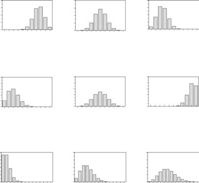
3.2.1 The Hypergeometric Distribution
The hypergeometric distribution arises when a random sample of size n is taken from a population of N units. If the population contains R units with a certain characteristic, then the probability that the sample will contain exactly x units with the characteristic is
P(x) = RC |
x |
N−RC /NC , for x = 0, 1, …, Min(n,R) |
(3.3) |
|
n−x n |
|
where aCb denotes the number of combinations of a objects taken b at a time. The proof of this result will be found in many elementary statistics texts. A
Models for Data |
63 |
random variable with the probabilities of different values given by equation (3.3) is said to have a hypergeometric distribution. The mean and variance are
μ = nR/N |
(3.4) |
and |
|
σ2 = [nR(N − R)(N − n)]/[N2 (N − 1)]. |
(3.5) |
As an example of a situation where this distribution applies, suppose that a grid is set up over a study area, and the intersection of the horizontal and vertical grid lines defines N possible sample locations. Let R of these locations have values in excess of a constant C. If a simple random sample of n of the N locations is taken, then equation (3.1) gives the probability that exactly x out of the n sampled locations will have a value exceeding C.
Figure 3.1(a) shows examples of probabilities calculated for some particular hypergeometric distributions.
3.2.2 The Binomial Distribution
Suppose that it is possible to carry out a certain type of trial and that, when this is done, the probability of observing a positive result is always p for each trial, irrespective of the outcome of any other trial. Then if n trials are carried out, the probability of observing exactly x positive results is given by the binomial distribution
P(x) = nCxpx(1 − p)n−x, for x = 0, 1, 2, …, n |
(3.6) |
which is a result also provided in Section A1.2 of Appendix 1. The mean and variance of this distribution are, respectively,
μ = np |
(3.7) |
and |
|
σ2 = np(1 − p). |
(3.8) |
An example of this distribution occurs with the situation described in Example 1.3, which was concerned with the use of mark–recapture methods to estimate survival rates of salmon in the Snake and Columbia Rivers in the Pacific Northwest of the United States. In that setting, if n fish are tagged and released into a river, and if there is a probability p of being recorded while passing a detection station downstream for each of the fish, then the probability of recording a total of exactly p fish downstream is given by equation (3.6).
Figure 3.1(b) shows some examples of probabilities calculated for some particular binomial distributions.
64 Statistics for Environmental Science and Management, Second Edition
P(x)
P(x)
P(x)
N = 40, R = 30, n = 10
0.4
0.3
0.2
0.1
0.0 0 2 4 6 8 10 x
n = 10, p = 0.2
0.4 |
|
|
|
|
|
|
0.2 |
|
|
|
|
|
|
0.0 |
0 |
2 |
4 |
6 |
8 |
10 |
|
||||||
|
|
|
|
x |
|
|
0.4 |
|
|
Mean = 1 |
|
||
|
|
|
|
|
|
|
0.3 |
|
|
|
|
|
|
0.2 |
|
|
|
|
|
|
0.1 |
|
|
|
|
|
|
0.0 |
0 |
3 |
|
6 |
9 |
12 |
|
|
|
|
x |
|
|
|
0.4 |
N = 40, R = 20, n = 10 |
0.4 |
N = 40, R = 10, n = 10 |
||||||||||
|
|
|
|
|
|
|
|
|
|
|
|
|
||
P(x) |
0.3 |
|
|
|
|
|
P(x) |
0.3 |
|
|
|
|
|
|
0.2 |
|
|
|
|
|
0.2 |
|
|
|
|
|
|
||
|
0.1 |
|
|
|
|
|
|
0.1 |
|
|
|
|
|
|
|
0.0 |
0 |
2 |
4 |
6 |
8 |
10 |
0.0 |
0 |
2 |
4 |
6 |
8 |
10 |
|
|
|
|
x |
|
|
|
|
|
|
x |
|
|
|
|
(a) Hypergeometric Distributions |
|
|
|
|
|
|
|
||||||
|
|
|
n = 10, p = 0.5 |
|
|
|
n = 10, p = 0.9 |
|
||||||
P(x) |
0.4 |
|
|
|
|
|
P(x) |
0.4 |
|
|
|
|
|
|
0.2 |
|
|
|
|
|
0.2 |
|
|
|
|
|
|
||
|
0.0 |
0 |
2 |
4 |
6 |
8 |
10 |
0.0 |
0 |
2 |
4 |
6 |
8 |
10 |
|
|
|
|
x |
|
|
|
|
|
|
x |
|
|
|
|
(b) Binomial Distributions |
|
|
|
|
|
|
|
||||||
|
0.4 |
|
|
Mean = 3 |
|
0.4 |
|
|
Mean = 5 |
|
|
|||
|
|
|
|
|
|
|
|
|
|
|
|
|
||
P(x) |
0.3 |
|
|
|
|
|
P(x) |
0.3 |
|
|
|
|
|
|
0.2 |
|
|
|
|
|
0.2 |
|
|
|
|
|
|
||
|
0.1 |
|
|
|
|
|
|
0.1 |
|
|
|
|
|
|
|
0.0 |
0 |
3 |
6 |
|
9 |
12 |
0.0 |
0 |
3 |
6 |
9 |
|
12 |
|
|
|
|
x |
|
|
|
|
|
|
x |
|
|
|
|
|
(c) Poisson Distributions |
|
|
|
|
|
|
|
|||||
Figure 3.1
Examples of hypergeometric, binomial, and Poisson discrete probability distributions.
3.2.3 The Poisson Distribution
One derivation of the Poisson distribution is as the limiting form of the binomial distribution as n tends to infinity and p tends to zero, with the mean μ = np remaining constant. More generally, however, it is possible to derive it as the distribution of the number of events in a given interval of time or a given area of space when the events occur at random, independently of each other at a constant mean rate. The probability function is
P(x) = exp(−μ)μx/x!, for x = 0, 1, 2, …, n |
(3.9) |
The mean and variance are both equal to μ.
In terms of events occurring in time, the type of situation where a Poisson distribution might occur is for counts of the number of occurrences of minor oil leakages in a region per month, or the number of cases per year of
Models for Data |
65 |
a rare disease in the same region. For events occurring in space, a Poisson distribution might occur for the number of rare plants found in randomly selected meter-square quadrats taken from a large area. In reality, though, counts of these types often display more variation than is expected for the Poisson distribution because of some clustering of the events. Indeed, the ratio of the variance of sample counts to the mean of the same counts, which should be close to 1 for a Poisson distribution, is sometimes used as an index of the extent to which events do not occur independently of each other.
Figure 3.1(c) shows some examples of probabilities calculated for some particular Poisson distributions.
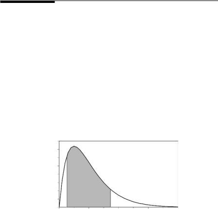
3.3 Continuous Statistical Distributions
Continuous distributions are often defined in terms of a probability density function, f(x), which is a function such that the area under the plotted curve between two limits a and b gives the probability of an observation within this range, as shown in Figure 3.2. This area is also the integral between a and b, so that, in the usual notation of calculus,
Prob(a < X < b) = ∫b |
f (x)dx |
(3.10) |
a |
|
|
The total area under the curve must be exactly 1, and f(x) must be greater than or equal to 0 over the range of possible values of x for the distribution to make sense.
f(x)
0.08
0.06
0.04
0.02
0.00 |
a |
1 |
b 2 |
3 |
4 |
0 |
x
Figure 3.2
The probability density function f(x) for a continuous distribution. The probability of a value between a and b is the area under the curve between these values, i.e., the area between the two vertical lines at x = a and x = b.