

1manly_b_f_j_statistics_for_environmental_science_and_managem
.pdf106Statistics for Environmental Science and Management, Second Edition
5.If the null hypothesis is true, then d1 should look like a typical value from the set of R differences, and is equally likely to appear anywhere in the list. On the other hand, if the two original samples
come from distributions with different means, then d1 will tend to be near the top of the list. On this basis, d1 is said to be significantly large at the 100α% level if it is among the top 100α% of values in the list. If 100α% is small (say 5% or less), then this is regarded as evidence against the null hypothesis.
It is an interesting fact that this test is exact in a certain sense even when R is quite small. For example, suppose that R = 99. Then, if the null hypoth-
esis is true and there are no tied values in the differences d1, d2, …, d100, the probability of d1 being one of the largest 5% of values (i.e., one of the largest 5)
is exactly 0.05. This is precisely what is required for a test at the 5% level, which is that the probability of a significant result when the null hypothesis is true is equal to 0.05.
The test just described is two-sided. A one-sided version is easily constructed by using the signed difference x − y as the test statistic, and seeing whether this is significantly large (assuming that the alternative to the null hypothesis of interest is that the values in the first sample come from a distribution with a higher mean than that for the second sample).
An advantage that the randomization approach has over a conventional parametric test on the sample mean difference is that it is not necessary to assume any particular type of distribution for the data, such as normal distributions for the two samples for a t-test. The randomization approach also has an advantage over a nonparametric test like the Mann-Whitney U-test because it allows the original data to be used rather than just the ranks of the data. Indeed, the Mann-Whitney U-test is really just a type of randomization test for which the test statistic only depends on the ordering of the data values in the two samples being compared.
A great deal more could be said about randomization testing, and much fuller accounts are given in the books by Edgington and Onghena (2007), Good (2004), and Manly (2007). The following example shows the outcome obtained on a real set of data.
Example 4.1: Survival of Rainbow Trout
This example concerns part of the results shown in Table 3.8 from a series of experiments conducted by Marr et al. (1995) to compare the survival of naive and metals-acclimated juvenile brown trout (Salmo trutta) and rainbow trout (Oncorhynchus mykiss) when exposed to a metals mixture with the maximum concentrations found in the Clark Fork River, Montana. Here only the results for the hatchery rainbow trout will be considered. For these, there were 30 control fish that were randomly selected to be controls and were kept in clean water for three weeks before being transferred to the metals mixture, while the remaining 29 fish were acclimated for three weeks in a weak solution of metals before being transferred to the stronger mixture. All the fish survived the initial three-week period,
Drawing Conclusions from Data |
107 |
and there is interest in whether the survival time of the fish in the stronger mixture was affected by the treatment.
In Example 3.2 the full set of data shown in Table 3.8 was analyzed using two-factor analysis of variance. However, a logarithmic transformation was first applied to the survival times to overcome the tendency for the standard deviation of survival times to increase with the mean. This is not that apparent when only the hatchery rainbow trout are considered. Therefore, if only these results were known, then it is quite likely that no transformation would be considered necessary. Actually, as will be seen shortly, it is immaterial whether a transformation is made or not if only these fish are considered.
Note that for this example, carrying out a test of significance to compare the two samples is reasonable. Before the experiment was carried out, it was quite conceivable that the acclimation would have very little, if any, effect on survival, and it is interesting to know whether the observed mean difference could have occurred purely by chance.
The mean survival difference (acclimated − control) is 10.904. Testing this using the randomization procedure using steps 1 to 5 described above using 4999 randomizations resulted in the observed value of 10.904 being the largest in the set of 5000 absolute mean differences consisting of itself and the 4999 randomized differences. The result is therefore significantly different from zero at the 0.02% level (1/5000). Taking logarithms to base 10 of the data and then running the test gives a mean difference of 0.138, which is again significantly different from zero at the 0.02% level. There is very strong evidence that acclimation affects the mean survival time, in the direction of increasing it.
Note that if it was decided in advance that, if anything, acclimation would increase the mean survival time, the randomization test could then be made one-sided to see whether the mean difference of (acclimated − control) is significantly large. This also gives a result that is significant at the 0.2% level using either the survival times or logarithms of these.
Note also that, in this example, the use of a randomization test is completely justified by the fact that the fish were randomly allocated to a control and to an acclimated group before the experiment began. This ensures that if acclimation has no effect, then the data that are observed are exactly equivalent to one of the alternative sets generated by randomizing this observed data. Any one of the randomized sets of data really would have been just as likely to occur as the observed set. When using a randomization test, it is always desirable that an experimental randomization be done to fully justify the test, although this is not always possible.
Finally, it is worth pointing out that any test on these data can be expected to give a highly significant result. A two-sample t-test using the mean survival times and assuming that the samples are from populations with the same variance gives t = 5.70 with 57 df, giving p = 0.0000. Using logarithms instead gives t = 5.39 still with 57 df and p = 0.0000. Using a Mann-Whitney U-test on either the survival times or logarithms also gives p = 0.0000. The conclusion is therefore the same, whatever reasonable test is used.

108 Statistics for Environmental Science and Management, Second Edition
4.7 Bootstrapping
Bootstrapping as a general tool for analyzing data was first proposed by Efron (1979). Initially, the main interest was in using this method to construct confidence intervals for population parameters using the minimum of assumptions, but more recently there has been increased interest in bootstrap tests of hypotheses (Efron and Tibshirani 1993; Hall and Wilson 1991; Manly 2007).
The basic idea behind bootstrapping is that when only sample data are available, and no assumptions can be made about the distribution that the data are from, then the best guide to what might happen by taking more samples from the distribution is provided by resampling the sample. This is a very general idea, and the way that it might be applied is illustrated by the following example.
Example 4.2: A Bootstrap 95% Confidence Interval
Table 3.3 includes the values for chlorophyll-a for 25 lakes in a region. Suppose that the total number of lakes in the region is very large and that there is interest in calculating a 95% confidence interval for the mean of chlorophyll-a, assuming that the 25 lakes are a random sample of all lakes.
If the chlorophyll-a values were approximately normally distributed, then this would probably be done using the t-distribution and equation (A1.9) from Appendix 1. The interval would then be
x − 2.064s/√25 < μ < x + 2.064s/√25 |
(4.2) |
where x is the sample mean, s is the sample standard deviation, and 2.064 is the value that is exceeded with probability 0.025 for the t-distribution with 24 df. For the data in question, x = 50.30 and s = 50.02, so the interval is
29.66 < μ < 70.95
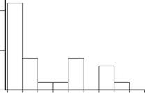
The problem with this is that the values of chlorophyll-a are very far from being normally distributed, as is clear from Figure 4.1. There is, therefore, a question about whether this method for determining the interval really gives the required level of 95% confidence.
Bootstrapping offers a possible method for obtaining an improved confidence interval, with the method that will now be described being called bootstrap-t (Efron 1981). This works by using the bootstrap to approximate the distribution of
t = (x − μ)/(s/√25)
instead of assuming that this follows a t-distribution with 24 df, which it would for a sample from a normal distribution. An algorithm to do this is as follows, where this is easily carried out in a spreadsheet.
Drawing Conclusions from Data |
109 |
Frequency
10
5
0
0 20 40 60 80 100 120 140 160 180 Chlorophyll-a
Figure 4.1
The distribution of chlorophyll-a for 25 lakes in a region, with the height of the histogram bars reflecting the percentage of the distribution in different ranges.
1.The 25 sample observations of chlorophyll-a from Table 3.3 are set up as the bootstrap population to be sampled. This population has the known mean of μB = 50.30.
2.A bootstrap sample of size 25 is selected from the population by making each value in the sample equally likely to be any of the 25 population values. This is sampling with replacement, so that a population value may occur 0, 1, 2, 3, or more times.
3.The t-statistic t1 = (x − μB)/(s/√25) is calculated from the bootstrap sample.
4.Steps 2 and 3 are repeated 5000 times to produce 5000 t-values t1, t2, …, t5000 to approximate the distribution of the t-statistic for samples from the bootstrap population.
5.Using the bootstrap distribution obtained, two critical values tlow and thigh are estimated such that
Prob[(x − μB)/(s/√25) < tlow] = 0.025
and
Prob[(x − μB)/(s/√25) > thigh] = 0.025
6.It is assumed that the critical values also apply for random samples of size 25 from the distribution of chlorophyll-a from which the original set of data was drawn. Thus it is asserted that
Prob[tlow < (x − μ)/(s/√25) < thigh] = 0.95
where x and s are now the values calculated from the original sample, and μ is the mean chlorophyll-a value for all lakes in the region of interest. Rearranging the inequalities then leads to the statement that
Prob[x − thighs/√25 < μ < x − tlows/√25] = 0.95
110 Statistics for Environmental Science and Management, Second Edition
Cumulative Probability
1.0
0.9
0.8
0.7
0.6
0.5
0.4
0.3
0.2
0.1
0.0
–5 |
–4 |
–3 |
–2 |
–1 |
0 |
1 |
2 |
3 |
4 |
5 |
|
|
|
|
|
t-Value |
|
|
|
|
|
|
|
Bootstrap Distribution |
t-Distribution with 24 df |
|
||||||
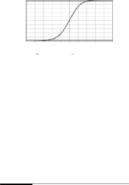
Figure 4.2
Comparison between the bootstrap distribution of (x − μB)/(s/√25) and the t-distribution with 24 df. According to the bootstrap distribution, the probability of a value less than tlow = −2.6 is approximately 0.025, and the probability of a value higher than thigh = 2.0 is approximately 0.025.
so that the required 95% confidence interval is
x − thighs/√25 < μ < x − tlows/√25 |
(4.3) |
The interval shown in equation (4.3) only differs from the usual confidence interval based on the t-distribution to the extent that tlow and thigh vary from 2.064. When the process was carried out, it was found that the bootstrap distribution of t = (x − μB)/(s/√25) is quite close to the t-distribu-
tion with 24 df, as shown by Figure 4.2, but with tlow = −2.6 and thigh = 2.0. Using the sample mean and standard deviation, the bootstrap-t interval
therefore becomes
50.30 − 2.0(50.02/5) < μ < 50.30 + 2.6(50.02/5)
or
30.24 < μ < 76.51
These compare with the limits of 29.66 to 70.95 obtained using the t-distribution. Thus the bootstrap-t method gives a rather higher upper limit, presumably because this takes better account of the type of distribution being sampled.
4.8 Pseudoreplication
The idea of pseudoreplication causes some concern, particularly among field ecologists, with the clear implication that when an investigator believes that replicated observations have been taken, this may not really be the case at
Drawing Conclusions from Data |
111 |
all. Consequently, there is some fear that the conclusions from studies will not be valid because of unrecognized pseudoreplication.
The concept of pseudoreplication was introduced by Hurlbert (1984) with the definition: “the use of inferential statistics to test for treatment effects with data from experiments where either treatments are not replicated, or replicates are not statistically independent.” Two examples of pseudoreplication are:
•a sample of meter-square quadrats randomly located within a 1-ha study region randomly located in a larger burned area is treated as a random sample from the entire burned area
•repeated observations on the location of a radio-tagged animal are treated as a simple random sample of the habitat points used by the animal, although in fact successive observations tend to be close together in space
In both of these examples it is the application of inferential statistics to dependent replicates as if they were independent replicates from the population of interest that causes the pseudoreplication. However, it is important to understand that using a single observation per treatment or per replicates that are not independent data is not necessarily wrong. Indeed it may be unavoidable in some field studies. What is wrong is to ignore this in the analysis of the data.
There are two common aspects of pseudoreplication. One of these is the extension of a statistical-inference observational study beyond the specific population studied to other unstudied populations. This is the problem with the first example above on the sampling of burned areas. The other aspect is the analysis of dependent data as if they are independent data. This is the problem with the example on radio-tagged animals.
When dependent data are analyzed as if they are independent, the sample size used is larger than the effective number of independent observations. This often results in too many significant results being obtained from tests of significance, and confidence intervals being narrower than they should be. To avoid this, a good rule to follow is that statistical inferences should be based on only one value from each independently sampled unit, unless the dependence in the data is properly handled in the analysis. For example, if five quadrats are randomly located in a study area, then statistical inferences about the area should be based on five values, regardless of the number of plants, animals, soil samples, etc., that are counted or measured in each quadrant. Similarly, if a study uses data from five radio-tagged animals, then statistical inferences about the population of animals should be based on a sample of size five, regardless of the number of times each animal is relocated.
When data are dependent because they are collected close together in time or space, there are a very large number of analyses available to allow for this. Many of these methods are discussed in later chapters in connection with

112 Statistics for Environmental Science and Management, Second Edition
particular types of applications, particularly in Chapters 8 and 9. For now, it is just noted that unless it is clearly possible to identify independent observations from the study design, then one of these methods needs to be used.
4.9 Multiple Testing
Suppose that an experimenter is planning to run a number of trials to determine whether a chemical at a very low concentration in the environment has adverse effects. A number of variables will be measured (survival times of fish, growth rate of plants, etc.) with comparisons between control and treated situations, and the experimenter will end up doing 20 tests of significance, each at the 5% level. He or she decides that if any of these tests give a significant result, then there is evidence of adverse effects. This experimenter then has a multiple testing problem.
To see this, suppose that the chemical has no perceptible effects at the level tested, so that the probability of a significant effect on any one of the 20 tests is 0.05. Suppose also that the tests are on independent data. Then the probability of none of the tests being significant is 0.9520 = 0.36, so that the probability of obtaining at least one significant result is 1 − 0.36 = 0.64. Hence the likely outcome of the experimenter’s work is to conclude that the chemical has an adverse effect even when it is harmless.
Many solutions to the multiple-testing problem have been proposed. The best known of these relate to the specific problem of comparing the mean values at different levels of a factor in conjunction with analysis of variance, as discussed in Section 3.5. There are also some procedures that can be applied more generally when several tests are to be conducted at the same time. Of these, the Bonferroni procedure is the simplest. This is based on the fact that if m tests are carried out at the same time using the significance level (100α%)/m, and if all of the null hypotheses are true, then the probability of getting any significant result is less than α. Thus the experimenter with 20 tests to carry out can use the significance level (5%)/20 = 0.25% for each test, and this ensures that the probability of getting any significant results is less than 0.05 when no effects exist.
An argument against using the Bonferroni procedure is that it requires very conservative significance levels when there are many tests to carry out. This has led to the development of a number of improvements that are designed to result in more power to detect effects when they do really exist. Of these, the method of Holm (1979) appears to be the one that is easiest to apply (Peres-Neto 1999). However, this does not take into account the correlation between the results of different tests. If some correlation does exist because the different test statistics are based partially on the same data, then, in principle, methods that allow for this should be better, such as the randomization procedure described by Manly (2007, sec. 6.8), which can be applied

Drawing Conclusions from Data |
113 |
in a wide variety of different situations (e.g., Holyoak and Crowley 1993), or several approaches that are described by Troendle and Legler (1998).
Holm’s method works using the following algorithm:
1.Decide on the overall level of significance α to be used (the probability of declaring anything significant when the null hypotheses are all true).
2.Calculate the p-value for the m tests being carried out.
3.Sort the p-values into ascending order, to give p1, p2, …, pm, with any tied values being put in a random order.
4.See if p1 ≤ α/m, and if so declare the corresponding test to give a significant result, otherwise stop. Next, see if p2 ≤ α/(m − 1), and if so declare the corresponding test to give a significant result, otherwise
stop. Next, see if p3 ≤ α/(m − 2), and if so declare the corresponding test to give a significant result, otherwise stop. Continue this process until an insignificant result is obtained, or until it is seen whether
pk ≤ α, in which case the corresponding test is declared to give a significant result. Once an insignificant result is obtained, all the remaining tests are also insignificant, because their p-values are at least as large as the insignificant one.
The procedure is illustrated by the following example.
Example 4.3: Multiple Tests on Characters for Brazilian Fish
This example to illustrate the Holm (1979) procedure is the one also used by Peres-Neto (1999). The situation is that five morphological characters have been measured for 47 species of Brazilian fish, and there is interest in which pairs of characters show significant correlation. Table 4.1 shows
Table 4.1
Correlations (r) between Characters for 47 Species of Brazilian Fish, with Corresponding p-Values
|
|
|
|
Character |
|
|
Character |
|
1 |
2 |
3 |
4 |
|
|
|
|
|
|
|
|
2 |
r |
0.110 |
… |
… |
… |
|
|
p-value |
0.460 |
… |
… |
… |
|
3 |
r |
0.325 |
0.345 |
… |
… |
|
|
p-value |
0.026 |
0.018 |
… |
… |
|
4 |
r |
0.266 |
0.130 |
0.142 |
… |
|
|
p-value |
0.070 |
0.385 |
0.340 |
… |
|
5 |
r |
0.446 |
0.192 |
0.294 |
0.439 |
|
|
p-value |
0.002 |
0.196 |
0.045 |
0.002 |
|
Note: For example, the correlation between characters 1 and 2 is 0.110, with p = 0.460.

114 Statistics for Environmental Science and Management, Second Edition
Table 4.2
Calculations and Results from the Holm Method for Multiple Testing Using the Correlations and p-Values from Table 4.1 and α = 0.05
i |
r |
p-Value |
0.05/(m + i – 1) |
Significance |
|
|
|
|
|
1 |
0.439 |
0.002 |
0.005 |
yes |
2 |
0.446 |
0.002 |
0.006 |
yes |
3 |
0.345 |
0.018 |
0.006 |
no |
4 |
0.325 |
0.026 |
0.007 |
no |
5 |
0.294 |
0.045 |
0.008 |
no |
6 |
0.266 |
0.070 |
0.010 |
no |
7 |
0.192 |
0.196 |
0.013 |
no |
8 |
0.142 |
0.340 |
0.017 |
no |
9 |
0.130 |
0.385 |
0.025 |
no |
10 |
0.110 |
0.460 |
0.050 |
no |
Source: Holm (1979).
the ten pairwise correlations obtained with their probability values based on the assumptions that the 47 species of fish are a random sample from some population, and that the characters being measured have normal distributions for this population. (For the purposes of this example, the validity of these assumptions will not be questioned.)
The calculations for Holm’s procedure, using an overall significance level of 5% (α = 0.05), are shown in Table 4.2. It is found that just two of the correlations are significant after allowing for multiple testing.
4.10 Meta-Analysis
The term meta-analysis is used to describe methods for combining the results from several studies to reach an overall conclusion. This can be done in a number of different ways, with the emphasis either on determining whether there is overall evidence of the effect of some factor, or of producing the best estimate of an overall effect.
A simple approach to combining the results of several tests of significance was proposed by Fisher (1970). This is based on three well-known results:
1.If the null hypothesis is true for a test of significance, then the p-value from the test has a uniform distribution between 0 and 1 (i.e., any value in this range is equally likely to occur).
2.If p has a uniform distribution, then −2loge(p) has a chi-squared distribution with 2 df.
3.If X1, X2, …, Xn all have independent chi-squared distributions, then their sum, S = ∑Xi, also has a chi-squared distribution, with the
Drawing Conclusions from Data |
115 |
number of degrees of freedom being the sum of the degrees of freedom for the components.
It follows from these results that if n tests are carried out on the same null hypothesis using independent data and yield p-values of p1, p2, …, pn, then a sensible way to combine the test results involves calculating
S1 =−2∑loge (pi ) |
(4.4) |
where this will have a chi-squared distribution with 2n degrees of freedom if the null hypothesis is true for all of the tests. A significantly large value of S1 is evidence that the null hypothesis is not true for at least one of the tests. This will occur if one or more of the individual p-values is very small, or if most of the p-values are fairly small.
There are a number of alternative methods that have been proposed for combining p-values, but Fisher’s method seems generally to be about the best, provided that the interest is in whether the null hypothesis is false for any of the sets of data being compared (Folks 1984). However, Rice (1990) argued that sometimes this is not quite what is needed. Instead, the question is whether a set of tests of a null hypothesis is in good agreement about whether there is evidence against the null hypothesis. Then a consensus p-value is needed to indicate whether, on balance, the null hypothesis is supported or not. For this purpose, Rice suggests using the Stouffer method described by Folks (1984).
The Stouffer method proceeds as follows. First, the p-value from each test is converted to an equivalent z-score, i.e., the p-value pi for the ith test is used to find the value zi such that
Prob(Z < zi) = pi |
(4.5) |
where Z is a random value from the standard normal distribution with a mean of 0 and a standard deviation of 1. If the null hypothesis is true for all of the tests, then all of the zi values will be random values from the standard normal distribution, and it can be shown that their mean z will be normally distributed with a mean of zero and a variance of 1/√n. The mean z-value can therefore be tested for significance by seeing whether
S2 = z/(1/√n) |
(4.6) |
is significantly less than zero.
There is a variation on the Stouffer method that is appropriate when, for some reason, it is desirable to weight the results from different studies differently. This weighting might, for example, be based on the sample sizes used in the study, some assessment of reliability, or perhaps with recent studies given the highest weights. This is called the Liptak-Stouffer method by Folks