1manly_b_f_j_statistics_for_environmental_science_and_managem

was upset to some extent. As a case study, the Exxon Valdez oil spill should, therefore, be a warning to those involved in oil spill impact assessment in the future about problems that are likely to occur with this type of design. Another aspect of these two studies that should give pause for thought is that the analyses that had to be conducted were rather complicated and might be difficult to defend in a court of law. They were not in tune with the KISS philosophy (Keep It Simple, Statistician).

Example 1.2:  Acid Rain in Norway

A Norwegian research program was started in 1972 in response to widespread concern in Scandinavian countries about the effects of acid precipitation (Overrein et al. 1980). As part of this study, regional surveys of small lakes were carried out from 1974 to 1978, with some extra sampling done in 1981. Data were recorded for pH, sulfate (SO4) concentration, nitrate (NO3) concentration, and calcium (Ca) concentration at each sampled lake. This can be considered to be a targeted study in terms of the three types of study that were previously defined, but it may also be viewed as a monitoring study that was only continued for a relatively short period of time. Either way, the purpose of the study was to detect and describe changes in the water chemical variables that might be related to acid precipitation.

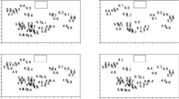
Table 1.1 shows the data from the study, as provided by Mohn and Volden (1985). Figure 1.2 shows the pH values, plotted against the locations of lakes in each of the years 1976, 1977, 1978, and 1981. Similar plots can be produced for sulfate, nitrate, and calcium. The lakes that were measured varied from year to year. There is, therefore, a problem with missing data for some analyses that might be considered.

In practical terms, the main questions that are of interest from this study are:

1.Is there any evidence of trends or abrupt changes in the values for one or more of the four measured chemistry variables?

2.If trends or changes exist, are they related for the four variables, and are they of the type that can be expected to result from acid precipitation?

Other questions that may have intrinsic interest and are also relevant to the answering of the first two questions are:

3.Is there evidence of spatial correlation such that measurements on lakes that are in close proximity tend to be similar?

4.Is there evidence of time correlation such that the measurements on a lake tend to be similar if they are close in time?

One of the important considerations in many environmental studies is the need to allow for correlation in time and space. Methods for doing this are discussed at some length in Chapters 8 and 9, as well as being mentioned briefly in several other chapters. Here it can merely be noted that a study of the pH values in Figure 1.2 indicates a tendency for the highest values to be in the north, with no striking changes from year to

10 Statistics for Environmental Science and Management, Second Edition

Figure 1.2

Values of pH for lakes in southern Norway in 1976, 1977, 1978, and 1981, plotted against the longitude and latitude of the lakes.

year for individual lakes (which are, of course, plotted at the same location for each of the years they were sampled).

Example 1.3:  Salmon Survival in the Snake River

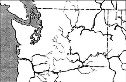
The Snake River and the Columbia River in the Pacific Northwest of the United States contain eight dams used for the generation of electricity, as shown in Figure 1.3. These rivers are also the migration route for hatchery and wild salmon, so there is a clear potential for conflict between different uses of the rivers. The dams were constructed with bypass systems for the salmon, but there has been concern nevertheless about salmon mortality rates in passing downstream, with some studies suggesting losses as high as 85% of hatchery fish in just portions of the river.

To get a better understanding of the causes of salmon mortality, a major study was started in 1993 by the National Marine Fisheries Service and the University of Washington to investigate the use of modern mark– recapture methods for estimating survival rates through both the entire river system and the component dams. The methodology was based on theory developed by Burnham et al. (1987) specifically for mark–­ recapture experiments for estimating the survival of fish through dams, but with modifications designed for the application in question (Dauble et al. 1993). Fish are fitted with passive integrated transponder (PIT) tags that can be uniquely identified at downstream detection stations in the bypass systems of dams. Batches of tagged fish are released, and their recoveries at detection stations are recorded. Using special probability models, it is then possible to use the recovery information to estimate the probability of a fish surviving through different stretches of the rivers and the probability of fish being detected as they pass through a dam.

In 1993 a pilot program of fish releases was conducted to (a) field-test the mark–recapture method for estimating survival, including testing

BRITISH COLUMBIA

Figure 1.3

Map of the Columbia River Basin showing the location of dams. Primary releases of pit-tagged salmon were made in 1993 and 1994 above Lower Granite Dam, with recoveries at Lower Granite Dam and Little Goose Dam in 1993, and at these dams plus Lower Monumental Dam in 1994.

the assumptions of the probability model; (b) identify operational and logistical constraints limiting the collection of data; and (c) determine whether survival estimates could be obtained with adequate precision. Seven primary batches of 830 to 1442 hatchery yearling chinook salmon (Oncorhynchus tshawytscha) were released above the Lower Granite Dam, with some secondary releases at Lower Granite Dam and Little Goose Dam to measure the mortality associated with particular aspects of the dam system. It was concluded that the methods used will provide accurate estimates of survival probabilities through the various sections of the Columbia and Snake Rivers (Iwamoto et al. 1994).

The study continued in 1994 with ten primary releases of hatchery yearling chinook salmon (O. tshawytscha) in batches of 542 to 1196, one release of 512 wild yearling chinook salmon, and nine releases of hatchery steelhead salmon (O. mykiss) in batches of 1001 to 4009, all above the first dam. The releases took place over a greater proportion of the juvenile migration period than in 1993, and survival probabilities were estimated for a larger stretch of the river. In addition, 58 secondary releases in batches of 700 to 4643 were made to estimate the mortality associated with particular aspects of the dam system. In total, the records for nearly 100,000 fish were analyzed, so that this must be one of the largest mark–recapture study ever carried out in one year with uniquely tagged individuals. From the results obtained, the researchers concluded that the assumptions of the models used were generally satisfied and reiterated their belief that these models permit the accurate estimation of survival probabilities through individual river sections, reservoirs, and dams on the Snake and Columbia Rivers (Muir et al. 1995).

12 Statistics for Environmental Science and Management, Second Edition

Table 1.2

Estimates of Survival Probabilities for 10 Releases of Hatchery Yearling Chinook Salmon Made above the Lower Granite Dam in 1994

Note: The survival is through the Lower Granite Dam, Little Goose Dam, and Lower Monumental Dam.

aThe standard errors shown with individual estimates are calculated from the mark-recapture model. The standard error of the mean is the standard deviation of the 10 estimates divided by √10.

Source: Muir et al. (1995).

In terms of the three types of studies that were defined previously, the mark–recapture experiments on the Snake River in 1993 and 1994 can be thought of as part of a baseline study, because the main objective was to assess this approach for estimating survival rates of salmon with the present dam structures, with a view to assessing the value of possible modifications in the future. Estimating survival rates for populations living outside captivity is usually a difficult task, and this is certainly the case for salmon in the Snake and Columbia Rivers. However, the estimates obtained by mark–recapture seem quite accurate, as indicated by the results shown in Table 1.2.

This example is unusual because of the use of the special mark–­ recapture methods. It is included here to illustrate the wide variety of statistical methods that are applicable for solving environmental problems, in this case improving the survival of salmon in a river that is used for electricity generation. More recent reports related to this example are provided by Williams et al. (2005) and Ferguson et al. (2005).

Example 1.4:  A Large-Scale Perturbation Experiment

Predicting the responses of whole ecosystems to perturbations is one of the greatest challenges to ecologists because this often requires experimental manipulations to be made on a very large scale. In many cases, small-scale laboratory or field experiments will simply not necessarily demonstrate the responses obtained in the real world. For this reason, a number of experiments have been conducted on lakes, catchments, streams, and open terrestrial and marine environments. Although these experiments involve little or no replication, they do indicate the response

potential of ecosystems to powerful manipulations that can be expected to produce massive unequivocal changes (Carpenter et al. 1995). They are targeted studies, as defined previously.

Carpenter et al. (1989) discussed some examples of large-scale experiments­ involving lakes in the Northern Highlands Lake District of Wisconsin. One such experiment, which was part of the Cascading Trophic Interaction Project, involved removing 90% of the piscivore biomass from Peter Lake and adding 90% of the planktivore biomass from another lake. Changes in Peter Lake over the following two years were then compared with changes in Paul Lake, which is in the same area but received no manipulation. Studies of this type are often referred to as having a before–after-control-impact (BACI) design, as discussed in Chapter 6.

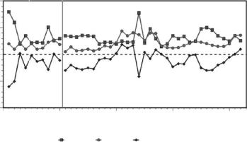
One of the variables measured at Peter Lake and Paul Lake was the chlorophyll concentration in mg/m3. This was measured for 10 samples taken in June to August 1984, for 17 samples taken in June to August 1985, and for 15 samples taken in June to August 1986. The manipulation of Peter Lake was carried out in May 1985. Figure 1.4 shows the results obtained. In situations like this, the hope is that time effects other than those due to the manipulation are removed by taking the difference between measurements for the two lakes. If this is correct, then a comparison between the mean difference between the lakes before the manipulation with the mean difference after the manipulation gives a test for an effect of the manipulation.

Before the manipulation, the sample size is 10 and the mean difference (treated-control) is −2.020. After the manipulation, the sample size is 32 and the mean difference is −0.953. To assess whether the change in the mean difference is significant, Carpenter et al. (1989) used a

Figure 1.4

The outcome of an intervention experiment in terms of chlorophyll concentrations (mg/m3). Samples 1 to 10 were taken in June to August 1984, samples 11 to 27 were taken from June to August 1985, and samples 28 to 42 were taken in June to August 1986. The treated lake received a food web manipulation in May 1985, between samples number 10 and 11 (as indicated by a vertical line).

14 Statistics for Environmental Science and Management, Second Edition

randomization test. This involved comparing the observed change with the distribution obtained for this statistic by randomly reordering the time series of differences, as discussed further in Section 4.6. The outcome of this test was significant at the 5% level, so they concluded that there was evidence of a change.

A number of other statistical tests to compare the mean differences before and after the change could have been used just as well as the randomization test. However, most of these tests may be upset to some extent by correlation between the successive observations in the time series of differences between the manipulated lake and the control lake. Because this correlation will generally be positive, it has the tendency to give more significant results than should otherwise occur. From the results of a simulation study, Carpenter et al. (1989) suggested that this can be allowed for by regarding effects that are significant between the 1% and 5% level as equivocal if correlation seems to be present. From this point of view, the effect of the manipulation of Peter Lake on the chlorophyll concentration is not clearly established by the randomization test.

This example demonstrates the usual problems with BACI studies. In particular:

1.the assumption that the distribution of the difference between Peter Lake and Paul Lake would not have changed with time in the absence of any manipulation is not testable, and making this assumption amounts to an act of faith; and

2.the correlation between observations taken with little time between them is likely to be only partially removed by taking the difference between the results for the manipulated lake and the control lake, with the result that the randomization test (or any simple alternative test) for a manipulation effect is not completely valid.

There is nothing that can be done about problem 1 because of the nature of the situation. More complex time series modeling offers the possibility of overcoming problem 2, but there are severe difficulties with using these techniques with the relatively small sets of data that are often available. These matters are considered further in Chapters 6 and 8.

Example 1.5:  Ring Widths of Andean Alders

Tree-ring width measurements are useful indicators of the effects of pollution, climate, and other environmental variables (Fritts 1976; Norton and Ogden 1987). There is, therefore, interest in monitoring the widths at particular sites to see whether changes are taking place in the distribution of widths. In particular, trends in the distribution may be a sensitive indicator of environmental changes.

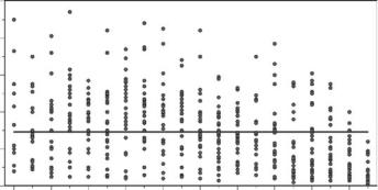
With this in mind, Dr. Alfredo Grau collected data on ring widths for 27 Andean alders (Alnus acuminanta) on the Taficillo Ridge at an altitude of about 1700 m in Tucuman, Argentina, every year from 1970 to 1989. The measurements that he obtained are shown in Figure 1.5. It is apparent here that, over the period of the study, the mean width decreased, as did the amount of variation between individual trees. Possible reasons

Figure 1.5

Tree-ring widths for Andean alders on Taficillo Ridge, near Tucuman, Argentina, 1970–1989. The horizontal line is the overall mean for all ring widths in all years.

for a change of the type observed here are climate changes and pollution. The point is that regularly monitored environmental indicators such as tree-ring widths can be used to signal changes in conditions. The causes of these changes can then be investigated in targeted studies.

Example 1.6:  Monitoring Antarctic Marine Life

An example of monitoring on a very large scale is provided by work carried out by the Commission for the Conservation of Antarctic Marine Living Resources (CCAMLR), an intergovernmental organization established to develop measures for the conservation of marine life of the Southern Ocean surrounding Antarctica. Currently 25 countries are members of the commission, while nine other states have acceded to the convention set up as part of CCAMLR to govern the use of the resources in question.

One of the working groups of CCAMLR is responsible for ecosystem monitoring and management. Monitoring in this context involves the collection of data on indicators of the biological health of Antarctica. These indicators are annual figures that are largely determined by what is available as a result of scientific research carried out by member states. They include such measures as the average weight of penguins when they arrive at various breeding colonies, the average time that penguins spend on the first shift incubating eggs, the catch of krill by fishing vessels within 100 km of land-based penguin breeding sites, average foraging durations of fur seal cows, and the percentage cover of sea ice. Major challenges in this area include ensuring that research groups of different nationalities collect data using the same standard methods and, in the longer term, being able to understand the relationships between different indicators and combining them better to measure the state of the Antarctic and detect trends and abrupt changes.