1manly_b_f_j_statistics_for_environmental_science_and_managem

16 Statistics for Environmental Science and Management, Second Edition

Example 1.7:  Evaluating the Attainment of Cleanup Standards

Many environmental studies are concerned with the specific problem of evaluating the effectiveness of the reclamation of a site that has suffered from some environmental damage. For example, a government agency might require a mining company to work on restoring a site until the biomass of vegetation per unit area is equivalent to what is found on undamaged reference areas. This requires a targeted study as defined previously.

There are two complications with using standard statistical methods in this situation. The first is that the damaged and reference sites are not generally selected randomly from populations of potential sites, and it is unreasonable to suppose that they would have had exactly the same mean for the study variable even in the absence of any impact on the damaged site. Therefore, if large samples are taken from each site, there will be a high probability of detecting a difference, irrespective of the extent to which the damaged site has been reclaimed. The second complication is that, when a test for a difference between the two sites does not give a significant result, this does not necessarily mean that a difference does not exist. An alternative explanation is that the sample sizes were not large enough to detect a difference that does exist.

These complications with statistical tests led to a recommendation by the U.S. Environmental Protection Agency (US EPA 1989a) that the null hypothesis for statistical tests should depend on the status of a site, in the following way:

1.If a site has not been declared to be contaminated, then the null hypothesis should be that it is clean, i.e., there is no difference from the control site. The alternative hypothesis is that the site is contaminated. A nonsignificant test result leads to the conclusion that there is no real evidence that the site is contaminated.

2.If a site has been declared to be contaminated, then the null hypothesis is that this is true, i.e., there is a difference (in an unacceptable direction) from the control site. The alternative hypothesis is that the site is clean. A nonsignificant test result leads to the conclusion that there is no real evidence that the site has been cleaned up.

The point here is that, once a site has been declared to have a certain status, pertinent evidence should be required to justify changing this status.

If the point of view expressed by items 1 and 2 is not adopted, so that the null hypothesis is always that the damaged site is not different from the control, then the agency charged with ensuring that the site is cleaned up is faced with setting up a maze of regulations to ensure that study designs have large enough sample sizes to detect differences of practical importance between the damaged and control sites. If this is not done, then it is apparent that any organization wanting to have the status of a site changed from contaminated to clean should carry out the smallest study possible, with low power to detect even a large difference from the control site. The probability of a nonsignificant test result (the site is clean) will then be as high as possible.

As an example of the type of data that may be involved in the comparison of a control site and a possibly contaminated one, consider some measurements of 1,2,3,4-tetrachlorobenzene (TcCB) in parts per

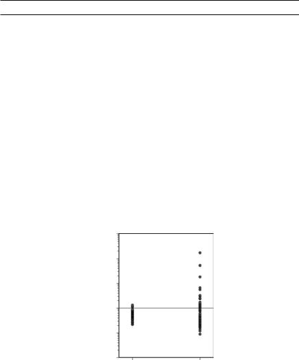
thousand million given by Gilbert and Simpson (1992, p. 6.22). There are 47 measurements made in different parts of the control site and 77 measurements made in different parts of the possibly contaminated site, as shown in Table 1.3 and Figure 1.6. Clearly the TcCB levels are much more

Table 1.3

Measurements of 1,2,3,4-Tetrachlorobenzene from Samples Taken at a Reference Site and a Possibly Contaminated Site

Reference Site (n = 47)

Figure 1.6

Comparison of TcCB measurements in parts per thousand million at a contaminated site (2) and a reference site (1).

18 Statistics for Environmental Science and Management, Second Edition

variable at the possibly contaminated site. Presumably, this might have occurred from the TcCB levels being lowered in parts of the site by cleaning, while very high levels remained in other parts of the site.

Methods for comparing samples such as these in terms of means and variation are discussed further in Chapter 7. For the data in this example, the extremely skewed distribution at the contaminated site, with several very extreme values, should lead to some caution in making comparisons based on the assumption that distributions are normal within sites.

Example 1.8:  Delta Smelt in the Sacramento–San Joaquin Delta

The final example considered in this chapter concerns the decline in the abundance of delta smelt (Hypomesus transpacificus) in the Sacramento– San Joaquin Delta in California, that apparently started in about 2000. The delta smelt is classified as a threatened species in the delta, so that there has been particular concern in the decline of this fish, although there is also evidence of the decline of other pelagic fish numbers at the same time.

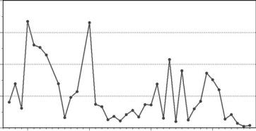
A number of surveys of the abundance of delta smelt take place each year. One of these surveys is called the fall midwater trawl, which samples adults over the four months September to December. From the survey results, an index of abundance is constructed by weighting the densities of fish observed in different parts of the delta by values that reflect the different amounts of habitats expected in those different regions. It is then assumed that the actual abundance of adult delta smelt in any year is proportional to the index value, at least approximately. Figure 1.7 shows the values of the fall midwater trawl index for the years since sampling began. The decline in numbers since 1999 is very clear.

There is much speculation about the cause of the decline in delta smelt numbers. Some claim that it is the result of the water being pumped out of the delta for use in towns and for agriculture, while others suggest

Figure 1.7

The fall midwater trawl abundance index for delta smelt for the years since sampling began in 1967, with no sampling in 1974 and 1979.

the whole season if this rate varies during the season. (Issues like this seem to come up with all studies in controversial areas.) Assuming that you know the likely length of the migration season, and roughly how many fish are likely to pass through the dam each week, how would you suggest that the average survival rate be estimated?

2

Environmental Sampling

2.1  Introduction

All of the examples considered in the previous chapter involved sampling of some sort, showing that the design of sampling schemes is an important topic in environmental statistics. This chapter is therefore devoted to considering this topic in some detail. The estimation of mean values, totals, and proportions from the data collected by sampling is covered at the same time, and this means that the chapter includes all methods that are needed for many environmental studies.

The first task in designing a sampling scheme is to define the population of interest as well as the sample units that make up this population. Here the population is defined as a collection of items that are of interest, and the sample units are these items. In this chapter it is assumed that each of the items is characterized by the measurements that it has for certain variables (e.g., weight or length), or which of several categories it falls into (e.g., the color that it possesses, or the type of habitat where it is found). When this is the case, statistical theory can assist in the process of drawing conclusions about the population using information from a sample of some of the items.

Sometimes defining the population of interest and the sample units is straightforward because the extent of the population is obvious, and a natural sample unit exists. At other times, some more-or-less arbitrary definitions will be required. An example of a straightforward situation is where the population is all the farms in a region of a country and the variable of interest is the amount of water used for irrigation on a farm. This contrasts with the situation where there is interest in the impact of an oil spill on the flora and fauna on beaches. In that case, the extent of the area that might be affected may not be clear, and it may not be obvious which length of beach to use as a sample unit. The investigator must then subjectively choose the potentially affected area and impose a structure in terms of sample units. Furthermore, there will not be one correct size for the sample unit. A range of lengths of beach may serve equally well, taking into account the method that is used to take measurements. The choice of what to measure will also, of course, introduce some further subjective decisions.

23

24 Statistics for Environmental Science and Management, Second Edition

2.2  Simple Random Sampling

A simple random sample is one that is obtained by a process that gives each sample unit the same probability of being chosen. Usually it will be desirable to choose such a sample without replacement so that sample units are not used more than once. This gives slightly more accurate results than sampling with replacement, whereby individual units can appear two or more times in the sample. However, for samples that are small in comparison with the population size, the difference in the accuracy obtained is not great.

Obtaining a simple random sample is easiest when a sampling frame is available, where this is just a list of all the units in the population from which the sample is to be drawn. If the sampling frame contains units numbered from 1 to N, then a simple random sample of size n is obtained without replacement by drawing n numbers one by one in such a way that each choice is equally likely to be any of the numbers that have not already been used. For sampling with replacement, each of the numbers 1 to N is given the same chance of appearing at each draw.

The process of selecting the units to use in a sample is sometimes facilitated by using a table of random numbers such as the one shown in Table 2.1. As an example of how such a table can be used, suppose that a study area is divided into 116 quadrats as shown in Figure 2.1, and it is desirable to select a simple random sample of ten of these quadrats without replacement. To do this, first start at an arbitrary place in the table such as the beginning of row five. The first three digits in each block of four digits can then be considered, to give the series 698, 419, 008, 127, 106, 605, 843, 378, 462, 953, 745, and so on. The first ten different numbers between 1 and 116 then give a simple random sample of quadrats: 8, 106, and so on. For selecting large samples, essentially the same process can be carried out on a computer using pseudo-random numbers in a spreadsheet, for example.

2.3  Estimation of Population Means

Assume that a simple random sample of size n is selected without replacement from a population of N units, and that the variable of interest has values y1, y2, …, yn, for the sampled units. Then the sample mean is

i=1

the sample variance is

Table 2.1

Random Number Table

Note: Each digit was chosen such that 0, 1, …, 9 were equally likely to occur. The grouping of four digits is arbitrary so that, for example, to select numbers from 0 to 99999, the digits can be considered five at a time.