

Baumgarten
.pdf64 3 Basic Equations
W |
|
ǻ |
w Wx1 x1 u1 Wx1 x2 u2 Wx1 x3 u3 |
|
w Wx2 x1 u1 Wx2 x2 u2 Wx2 x3 u3 |
|
|||||||
|
|
|
|
||||||||||
W |
|
« |
|
wx |
|
|
|
|
wx |
|
|
|
|
|
|
¬ |
|
1 |
|
|
|
|
|
2 |
|
|
|
|
|
|
|
|
|
|
|
|
|
|
(3.68) |
||
|
|
w Wx3 x1 u1 Wx3 x2 u2 Wx3 x3 u3 |
ȼ |
|
|
|
|
||||||
|
|
|
|
& |
|
|
|
||||||
|
|
|
|
wx |
|
|
dx dx dx |
= |
u |
T |
dx dx dx . |
||
|
|
|
|
» |
1 2 3 |
|
|
W |
1 2 3 |
||||
|
|
|
|
3 |
¼ |
|
|
|
|
|
|
||
|
|
|
|
|
|
|
|
|
|
|
|||
The change of energy due to the effect of body forces is |
|
|
|||||||||||
|
|
|
|
Wg |
& |
|
|
|
|
|
|
|
|
|
|
|
|
f u& dx1dx2 dx3 |
, |
|
|
(3.69) |
|||||
where |
& |
|
Ug& |
in the case of gravitation. |
|
|
|
|
|
||||
f |
|
|
|
|
|
|
|||||||
Using Eqs. 3.61, 3.64, 3.67, 3.68, and 3.69 in Eq. 3.59 and applying the product rule results in
§ |
|
|
u& |
|
2 ·§wU |
|
w Uu1 |
|
|
w Uu2 |
|
|
|
w Uu3 |
· |
|
De |
|||||||
|
|
|
|
|||||||||||||||||||||
¨e |
|
|
|
|
|
¸ |
|
|
|
|
|
|
|
|
|
|
|
|
|
|
U |
|
|
|
|
|
|
|
|
¨ wt |
wx |
|
wx |
|
|
wx |
|
¸ |
Dt |
||||||||||
¨ |
|
2 ¸ |
|
|
|
|
|
|
|
|
||||||||||||||
© |
|
¹ |
© |
|
|
1 |
|
|
2 |
|
|
3 |
|
¹ |
|
|
|
|||||||
|
|
|
|
|
|
|
|
|
|
& |
|
|
& |
|
|
& & |
|
|
|
Q |
|
|
||
O T pu u TW f u |
|
|
|
s |
|
|
||||||||||||||||||
dx1dx2dx3 |
||||||||||||||||||||||||
|
|
|
|
|
|
|
|
|
|
|
|
|
|
|
|
|
|
|||||||
U |
D |
§ |
|
u& |
|
2 · |
||
|
|
|||||||
|
¨ |
|
|
|
|
|
¸ |
|
|
|
|
|
|
|
|||
|
2 |
|||||||
|
Dt ¨ |
¸ |
||||||
|
|
© |
|
|
|
|
|
¹ |
.
(3.70)
Because of the continuity equation, the first term in Eq. 3.70 is zero. The use of
|
|
|
|
|
|
|
|
|
& |
|
& |
|
|
|
wu j |
|
|
|
|||
|
|
|
|
|
|
|
u |
TW |
u TW Wij |
|
|
|
|
|
(3.71) |
||||||
|
|
|
|
|
|
wx |
|
|
|
|
|||||||||||
|
|
|
|
|
|
|
|
|
|
|
|
|
|
|
|
i |
|
|
|
||
and |
|
|
|
|
|
|
|
|
|
|
|
|
|
|
|
|
|
|
|
|
|
|
|
|
|
|
|
|
|
|
pu& p u& u& p |
|
|
(3.72) |
|||||||||
results in: |
|
|
|
|
|
|
|
|
|
|
|
|
|
|
|
|
|
|
|
|
|
§ |
De |
|
D |
§ |
|
u& |
|
2 ·· |
|
& |
|
& |
|
|
|
|
|
||||
|
|
|
|
|
|
|
|
|
|
||||||||||||
U ¨ |
|
|
|
¨ |
|
|
|
|
|
¸¸ |
O T p u |
u p |
|
|
|
||||||
Dt |
|
2 |
|
|
|
|
|||||||||||||||
¨ |
|
Dt ¨ |
¸¸ |
|
|
|
|
|
|
|
|
|
|
|
|||||||
© |
|
|
|
© |
|
|
|
|
¹¹ |
|
|
|
|
|
|
|
|
|
|
|
|
|
|
|
|
|
|
|
|
|
|
|
& |
|
wu j |
|
& & |
|
Q |
|
|||
|
|
|
|
|
|
|
|
|
|
|
u TW Wij |
|
|
|
|
|
|
s |
|
||
|
|
|
|
|
|
|
|
|
|
|
|
|
f u |
|
. |
|
|||||
|
|
|
|
|
|
|
|
|
|
|
wx |
|
dx dx dx |
(3.73) |
|||||||
|
|
|
|
|
|
|
|
|
|
|
|
|
i |
|
1 |
2 3 |
|
||||
This equation is further modified by using the momentum equation. Multiplication of Eq. 3.49 with the velocity vector yields the second term on the left hand side of Eq. 3.73,
3.1 Description of the Continuous Phase |
65 |
|
|
& Du& |
|
D |
§ |
|
|
u& |
|
2 · |
& |
& |
& & |
|
|
||
|
|
|
|
|
|||||||||||
Uu |
|
U |
|
¨ |
|
|
|
|
|
¸ |
u |
p u |
TW u f |
, |
(3.74) |
Dt |
|
|
2 |
||||||||||||
|
|
Dt ¨ |
¸ |
|
|
|
|
|
|||||||
|
|
|
|
© |
|
|
|
|
|
¹ |
|
|
|
|
|
and Eq. 3.73 now reads
|
De |
& |
wu j |
|
Q |
|
|
U |
|
O T p u Wij |
|
|
s |
, |
(3.75) |
Dt |
wx |
dx dx dx |
|||||
|
|
|
i |
1 2 3 |
|
|
|
which is a widely used form of the first law of thermodynamics for fluid motion, the so-called thermal energy equation. In the case of a Newtonian fluid, the components of the stress tensor can be expressed by Eq. 3.51. This finally yields
|
|
|
De |
|
|
|
|
|
|
|
|
|
|
|
|
|
|
|
|
& |
|
|
|
|
|
|
|
|
|
|
Q |
|
|
|
|
|
|
||||
|
U |
|
|
|
|
O T p u µ) |
|
|
|
|
s |
|
|
, |
|
(3.76) |
|||||||||||||||||||||||||
|
Dt |
|
dx1dx2 dx3 |
|
|||||||||||||||||||||||||||||||||||||
|
|
|
|
|
|
|
|
|
|
|
|
|
|
|
|
|
|
|
|
|
|
|
|
|
|
|
|
|
|
|
|
||||||||||
where |
|
|
|
|
|
|
|
|
|
|
|
|
|
|
|
|
|
|
|
|
|
|
|
|
|
|
|
|
|
|
|
|
|
|
|
|
|
|
|
|
|
|
ªw2u |
|
w2u |
|
|
w2u |
|
º §wu |
2 |
|
|
|
wu ·2 |
|
|
|
|
|
|
|
|
||||||||||||||||||||
) 2 |
« |
|
|
|
1 |
|
|
|
|
2 |
|
|
|
|
3 |
|
» |
¨ |
|
|
|
|
|
1 |
¸ |
|
|
|
|
|
|
|
|
|
|||||||
|
|
|
2 |
|
wx |
2 |
|
|
wx |
2 |
|
|
|
|
|
|
|
|
|
|
|
|
|
|
|
|
|
||||||||||||||
|
« wx |
|
|
|
|
|
|
|
|
|
|
» |
© wx1 |
|
|
|
wx2 ¹ |
|
|
|
|
|
|
|
|
||||||||||||||||
|
¬ |
|
1 |
|
|
|
2 |
|
|
3 |
|
¼ |
|
|
|
|
|
|
|
|
|
|
|
|
|
|
|
|
|
|
|
|
|
|
|||||||
§wu |
3 |
|
|
|
wu |
2 |
·2 §wu |
|
|
|
|
wu |
3 |
·2 |
|
|
2 §wu |
|
wu |
2 |
|
|
wu |
·2 |
|
||||||||||||||||
+¨ |
|
|
|
|
|
|
¸ |
|
¨ |
|
1 |
|
|
|
¸ |
|
|
|
|
¨ |
|
1 |
|
|
|
|
|
3 |
¸ |
|
|||||||||||
|
|
|
|
|
|
|
|
|
|
|
|
3 |
|
|
|
|
|
|
(3.77) |
||||||||||||||||||||||
© wx2 |
|
|
wx3 ¹ |
|
|
©wx3 |
|
|
wx1 ¹ |
|
|
|
© wx1 |
|
wx2 |
|
wx3 ¹ |
||||||||||||||||||||||||
is the dissipation function.
Eq. 3.76 may be rearranged in order to get an expression based on the enthalpy h. The continuity equation (Eq. 3.40) can be rewritten to give
& |
|
|
p DU |
|
D § p · |
|
Dp |
|
|
|||||
p u |
|
|
|
|
|
U |
|
¨ |
|
¸ |
|
|
. |
(3.78) |
U |
|
Dt |
|
|
Dt |
|||||||||
|
|
|
|
|
Dt © |
U ¹ |
|
|
|
|||||
Combining Eqs. 3.78 and 3.76 and neglecting the source term Qs yields
|
D § |
p · |
|
Dh |
|
Dp |
O T µ) . |
|
||
U |
|
¨e |
|
¸ |
U |
|
|
|
(3.79) |
|
|
|
Dt |
|
Dt |
||||||
|
Dt © |
U ¹ |
|
|
|
|
||||
The dissipation term can usually be neglected. This term becomes important for high Mach number flows (e.g. reentry of a spacecraft into the earth’s atmosphere). Assuming that the thermal conductivity and the specific heat capacity are constants and neglecting the usually small effect of the pressure term on temperature results in the following often used form of the thermal energy equation:
Uc |
|
DT |
Uc |
§wT |
u |
|
wT · |
O |
w2T |
. |
(3.80) |
||
p |
Dt |
p ¨ |
wt |
i |
|
¸ |
2 |
||||||
|
|
|
© |
|
|
wxi ¹ |
|
wxi |
|
|
|||
66 3 Basic Equations
3.1.4 Turbulent Flows
3.1.4.1 RANS Equations
The Navier-Stokes equations can be solved directly without averaging or using turbulence models if the grid spacing is fine enough to resolve the smallest eddies in a flow field. This approach is called direct numerical simulation (DNS). The size of the smallest eddies is proportional to the Kolmogorov length scale, which decreases with increasing Reynolds numbers. For a cylinder volume of 1.0 liters at least 1012 grid points are needed due to the highly turbulent flow, where the smallest eddies are in the range of 0.01 mm. The requirements for the application of DNS to in-cylinder processes, concerning computer speed and memory, exceed the power of today’s processors by far. Up to now, DNS simulations have not been suitable for solving engineering problems and are limited to basic research applications with low Reynolds numbers and small geometric domains.
The large eddy simulation (LES) distinguishes between large and small eddies. Only the large eddies, which contain most of the energy and thus are much more important concerning the transport of the conserved quantities than the small ones, are resolved by the grid. The effect of the small eddies is described by sub-models. The separation of small and large eddies is obtained by filtering the flow field using an appropriate threshold value of the eddy size. Because the small eddies are described by so-called subgrid-scale Reynolds stress models, the Navier–Stokes equations are expressed in terms of averaged quantities, similar to the RANS equations described in the following. The numerical algorithms are usually specially adapted to the individual problem and the geometry. Although the large eddy simulation consumes less time and computational power than DNS, it is still not suitable for engineering applications. A more detailed description of DNS and LES is given in [6] for example.
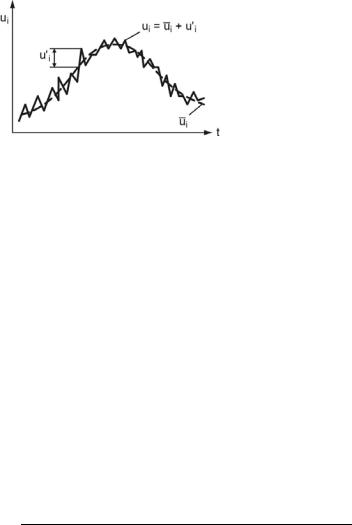
Today, the computation of technical flow fields is performed using the socalled Reynolds averaged Navier-Stokes equations (RANS equations) in combination with an appropriate turbulence model. Following the basic approach of Reynolds (1895), the instantaneous values of the turbulent flow quantities are split into a mean and a fluctuating component (Reynolds decomposition):
ui |
ui uic , U |
|
|
|
|
(3.81) |
|
Uc , T T T c . |
|||||
U |
||||||
The overbar denotes the time-average, and the superscript (´) denotes the superimposed fluctuation, see Fig. 3.9. The time-average of a flow quantity, e.g. a velocity component, is
|
|
1 t 't |
|
& |
|
|
||
u |
|
|
³ |
u |
x,t dt . |
(3.82) |
||
i 't |
||||||||
|
i |
|
|
|||||
|
|
|
t |
|
|
|
|
|
The time interval t must be large compared to the relevant period of the fluctuations, but small enough to map the time dependence of an unsteady mean flow.
3.1 Description of the Continuous Phase |
67 |
|
|
Fig. 3.9. Unsteady turbulent flow
The RANS equations are obtained by substituting the Reynolds decomposition terms into the instantaneous conservation equations, and then by averaging the entire equations over time. Now the turbulent flow is described by the conservation equations in terms of time average quantities. Due to the time-averaging, the information about the turbulent fluctuating quantities is lost. This effect is shown in additional terms in the momentum and energy equations, the Reynolds stresses, and the turbulent heat flux, which have to be described by a turbulence model in order to close the system of equations again.
In general, thermodynamic properties like Π, cp, and Ο can also fluctuate due to the fluctuation of pressure and temperature, but these fluctuations are usually small, and they are neglected for the treatment of turbulence in this book. Special attention must be given to the density fluctuations. Neglecting the density fluctuations does not mean that the density is constant. It simply expresses the fact that the effect of turbulent density variations is not included; the mean density variations however may be large. Should fluctuations in density be considered, the appropriate equations can be derived either by simple time-averaging (Reynolds averaging, Eq. 3.81), or by a mass-weighted time-averaging procedure (Favreaveraging). Both kinds of averaging are in use today and will be described in the following.
Substituting the Reynolds decomposition terms into the instantaneous continuity equation (here only shown for two-dimensional flow) and averaging over time (denoted by a long overbar) yields
|
|
w |
|
|
Uc |
w |
|
» |
|
Uc u1 u1c ¼º |
w |
» |
|
Uc |
|
2 u2c ¼º 0 . |
||||||||||||||||||||||||||
|
U |
|
U |
U |
u |
|||||||||||||||||||||||||||||||||||||
|
wt |
wx |
|
wx |
||||||||||||||||||||||||||||||||||||||
1 |
|
|
|
|
|
|
|
|
|
|
|
|
|
|
2 |
|
|
|
|
|
|
|
|
|
|
|
|
|
|
|
||||||||||||
By applying the following rules of averaging (e.g. [20, 11]), |
||||||||||||||||||||||||||||||||||||||||||
|
|
|
0 , |
|
|
|
, |
|
|
|
|
|
|
|
g , |
|
|
0 , |
|
|
|
|
|
|
g , |
|||||||||||||||||
|
|
|
|
|
|
|
|
|
|
|
|
|
|
|
|
|
|
|
|
|
|
|||||||||||||||||||||
|
|
f c |
f g |
f c g |
f g |
|||||||||||||||||||||||||||||||||||||
|
|
f |
f |
f |
f |
|||||||||||||||||||||||||||||||||||||
|
|
|
|
|
|
|
|
|
|
|
|
|
|
|
|
|
|
|
|
|
|
|
|
|
|
w |
|
|
|
|
|
|
|
|
||||||||
|
|
|
|
|
|
|
|
|
|
|
|
|
|
|
|
|
|
|
|
|
|
|
|
wf |
|
|
|
|
|
|
|
|
|
|||||||||
|
|
|
|
|
|
|
|
|
|
|
|
|
|
|
|
|
|
|
g |
|
, |
|
|
|
|
f |
|
|
|
|
|
|
|
|
||||||||
|
|
|
|
|
|
|
|
|
|
|
|
|
f g |
f c gc |
|
|
|
, |
|
|
|
|
|
|||||||||||||||||||
|
|
|
|
|
|
|
|
|
|
|
|
|
|
|
f |
|
|
|
|
|
|
|
|
|||||||||||||||||||
|
|
|
|
|
|
|
|
|
|
|
|
|
|
|
|
|
ws |
|
|
ws |
|
|
|
|
|
|
||||||||||||||||
|
|
|
|
|
|
|
|
|
|
|
|
|
|
|
|
|
|
|
|
|
|
|
|
|
|
|
|
|
|
|
|
|
|
|
|
|
||||||
(3.83)
(3.84)
where f and g are two turbulent flow quantities, the continuity equation for a compressible flow becomes
68 3 Basic Equations
w |
U |
|
|
w |
|
|
|
|
w |
|
|
|
|
|
w |
|
|
|
w |
|
|
|
|
|
|
|
|
|
|
|
|
|
|
|
Ucu1c |
Ucu2c 0 . |
|
||||||||||
|
|
|
|
|
U |
u1 |
|
U |
u |
2 |
|
|
(3.85) |
||||||||||
wt |
|
wx |
wx |
wx |
wx |
||||||||||||||||||
|
|
1 |
2 |
1 |
2 |
|
|
|
|
||||||||||||||
Compared to the original continuity equation, there are additional terms expressing the fact that the mean flow quantities alone no longer express the mass conservation principle. For incompressible (constant density) flow, the fluctuation terms disappear, and the continuity equation reduces to
w |
|
|
|
|
|
ui |
0 . |
(3.86) |
|||
wxi |
|||||
|
|
||||
The momentum and energy equations are treated accordingly. Replacing the instantaneous values by the Reynolds decompositions, averaging over time, separating components, and dropping all terms that contain only one fluctuating quantity (these terms are zero), the x1-momentum equation for a compressible flow in the absence of external forces becomes (here only shown for two-dimensional flow)
w |
|
|
|
|
|
|
|
|
|
|
w |
|
|
u12 |
|
w |
|
|
|
|
|
|
2 |
w |
|
|
|
|
|
|
|
|
w |
|
|
|
|
|
|
|
||||||||||||||||||
|
|
u1 |
|
|
|
|
|
|
|
|
u1 |
|
|
|
u1c2 |
|||||||||||||||||||||||||||||||||||||||||||
|
|
Ucu1c |
u1cu2c |
|||||||||||||||||||||||||||||||||||||||||||||||||||||||
U |
U |
|
U |
u |
U |
U |
||||||||||||||||||||||||||||||||||||||||||||||||||||
wt |
wx |
wx |
wx |
wx |
||||||||||||||||||||||||||||||||||||||||||||||||||||||
|
|
|
|
|
|
|
|
|
|
|
|
|
|
|
|
1 |
|
|
|
|
2 |
|
1 |
2 |
|
|
|
|
|
|
|
|
||||||||||||||||||||||||||
|
w |
|
|
|
w |
|
|
|
|
|
|
w |
2u1 |
|
|
w |
|
|
|
|
|
2 |
|
|
||||||||||||||||||||||||||||||||||
|
|
Ucu1c2 |
||||||||||||||||||||||||||||||||||||||||||||||||||||||||
|
|
Ucu1cu2c |
Ucu1c |
u |
Ucu2c |
u |
Ucu1c |
|||||||||||||||||||||||||||||||||||||||||||||||||||
wx |
wx |
|
wx |
wx |
||||||||||||||||||||||||||||||||||||||||||||||||||||||
|
|
|
1 |
|
|
|
|
|
|
|
|
|
|
2 |
|
|
|
|
|
|
|
|
1 |
|
|
|
|
|
|
|
|
|
2 |
|
|
|
|
|
|
|
|
|
|
|
|
|
|
|
|
|||||||||
|
|
|
|
wp |
|
|
|
|
x1 x1 |
|
|
|
|
x2 x1 |
|
|
|
|
|
|
|
|
|
|
|
|
|
|
|
|
|
|
|
|
|
|
|
|
|
|
|
|
|
|
|
|
||||||||||||
|
|
+ |
wW |
|
wW |
. |
|
|
|
|
|
|
|
|
|
|
|
|
|
|
|
|
|
|
|
|
|
|
|
|
|
|
|
|
|
|
|
|||||||||||||||||||||
wx1 |
wx1 |
|
wx2 |
|
|
|
|
|
|
|
|
|
|
|
|
|
(3.87) |
|||||||||||||||||||||||||||||||||||||||||
|
|
|
|
|
|
|
|
|
|
|
|
|
|
|
|
|
|
|
|
|
|
|||||||||||||||||||||||||||||||||||||
The fluctuating parts of the viscous stress tensor disappear entirely upon timeaveraging. The x2- and x3- momentum equations as well as the energy equation may be treated in the same manner. Compared to the original equations, there are again a lot of extra terms due to additional turbulent momentum and heat transfer, complicating the system of conservation equations.
In the case of incompressible flow however, the resulting momentum and energy conservation equations reduce to
§w |
u |
j |
|
|
|
|
|
wu j · |
wp |
|
w |
|
|
|
|
|
|
|
||||||||
|
|
|
|
|
|
|
|
|
|
|
|
|
||||||||||||||
U ¨ |
|
ui |
|
¸ |
|
|
|
|
|
|
Wij Uuicucj , |
|||||||||||||||
wt |
wx |
wx |
j |
wx |
||||||||||||||||||||||
© |
|
|
|
|
|
|
|
|
i |
¹ |
|
|
|
|
i |
|
|
|
|
|
|
|
||||
|
|
|
|
|
|
|
|
|
|
|
|
|
|
|
|
|
|
|
|
|
|
|
|
|||
|
|
§wT |
|
|
wT |
· |
|
|
w |
|
|
|
|
|
|
|
|
|
||||||||
|
|
|
|
|
|
|
|
|
|
Ucp uicT c , |
||||||||||||||||
|
|
|
|
|
|
|
|
|
|
|
|
|
|
|
|
|||||||||||
Ucp ¨ |
wt |
|
ui wx ¸ |
wx |
||||||||||||||||||||||
qi |
||||||||||||||||||||||||||
|
© |
|
|
|
|
|
|
|
i ¹ |
|
|
i |
|
|
|
|
|
|
|
|
|
|
||||
(3.88)
(3.89)
where j = 1, 2, 3 indicates that there are three momentum equations, each for one coordinate direction. These equations are very similar to the original set of conservation equations. However, two additional terms have been added as a result of the averaging process. In the momentum equation, this is the so-called turbulent stress tensor,

|
|
|
3.1 Description of the Continuous Phase |
69 |
|
|
|
|
|
|
|
|
|
|
|||
|
|
|
|
|
|
Wij ,t Uuicucj |
(3.90) |
||||
(with the minus sign dropped it is called Reynolds stress tensor), and in the energy equation there is the turbulent heat flux,
|
Ucp uicT c . |
(3.91) |
qi,t |
The Reynolds stress term is not a stress but an inertia effect due to additional momentum exchange caused by turbulence and is only referred to as a stress because of the way it appears in the equations. The same holds true for the turbulent heat flux: this term represents the increase of heat transfer due to the presence of turbulent eddies.
Altogether, is has been shown that, except for the turbulent stresses and the turbulent heat flux, the RANS equations for incompressible flow have the same form as the original conservation equations. In the case of fully compressible flow however, the equations are much more complicated.
For this reason, the conservation equations for compressible turbulent flows are often obtained by a mass-weighted time-averaging procedure according to A. Favre (1965) (e.g. Cebeci and Smith [4] and Oertel [16]). Favre-averaging results in conservation equations which are very similar to the original ones, and which contain only few additional terms due to the effect of turbulence.
Favre-averaging of a flow quantity, e.g. the velocity component ui, is obtained by dividing the time-averaged product of density and velocity,
|
|
|
1 |
t 't |
|
|
||||
|
|
|
³ pui dt , |
|
||||||
|
pui |
(3.92) |
||||||||
|
|
't |
||||||||
|
|
|
|
|
t |
|
|
|||
by the time-averaged density: |
|
|
|
|
|
|
|
|||
|
|
|
|
|
|
|
|
|
|
|
|
|
|
Uui |
|
|
|||||
|
|
|
|
|
|
|
||||
|
|
ui |
|
|
U |
. |
(3.93) |
|||
|
|
|
|
|
|
|
|
|||
The instantaneous flow quantities are again split into a mean value, denoted by (~), and a fluctuating value, denoted by (´´). This is done for all flow quantities except for static pressure and the density, which are only time-averaged:
|
|
|
|
|
|
|
U U Uc , p p pc , ui |
ui uicc , |
(3.94) |
||||
T T T cc . |
||||||
|
|
|
|
|
|
|
In contrast to the fluctuation components of the simple Reynolds decompositions ( uiχ ), the time average of the Favre-averaged fluctuation components (uiχχ) is not
zero. Instead |
Υuiχχ 0 , which can be shown by the following calculation: |
|
|||||||||||||||||||||||||||||||||||
|
|
|
|
|
|
|
|
|
|
|
|
|
|
|
|
|
|
|
|
|
|
|
|
|
|
|
|
|
|
|
|
|
|
|
|
|
|
|
|
Uui |
|
|
|
|
Uuicc |
|
|
|
|
|
|
Uuicc |
|
Uuicc |
|
|
|||||||||||||||||||
|
|
|
|
|
|
|
|
|
|
|
|
||||||||||||||||||||||||||
|
|
|
|
Uui |
|
|
Uui |
|
|
|
|
|
|||||||||||||||||||||||||
|
|
|
|
|
|
|
|
|
|
|
|
|
|
|
|
|
|||||||||||||||||||||
|
|
|
|
|
|
|
|
|
|
|
|
|
|
|
|
|
|
|
|
|
|
|
|
|
|
|
ui |
|
|
|
|
. |
(3.95) |
||||
|
|
U |
U |
U |
U |
U |
U |
||||||||||||||||||||||||||||||
Because ui |
|
/ U |
by definition, the last term in Eq. 3.95 is zero. |
|
|||||||||||||||||||||||||||||||||
Uui |
|
||||||||||||||||||||||||||||||||||||
|
|
|
|
|
|
|
|
|
|
|
|
|
|
|
|
|
|
|
|
|
|
|
|
|
|
|
|
|
|
|
|
|
|
|
|
|
|
70 3 Basic Equations
Using the following rules of averaging, |
|
|
|
|
|
|
|
|
|
|
|
|
|
|
|
|
|
||||||||||||||||||
|
|
|
|
|
|
|
|
|
|
|
|
|
|
|
|
|
|
|
|
|
|
|
|
|
|
|
|
|
ω |
|
|
|
|
|
|
|
|
|
|
|
|
|
|
|
|
|
|
|
|
|
|
|
|
|
|
|
|
|
|
ωf |
|
|
|||||||||
|
|
|
|
|
|
|
|
|
|
|
|
|
|
|
|
|
|
|
|
|
|
|
|
|
f |
|
|||||||||
|
|
|
|
|
|
|
|
|
|
|
|
|
|
|
|
|
|
|
|
||||||||||||||||
|
|
|
|
|
f g |
|
|
|
f g , |
|
0 , |
(3.96) |
|||||||||||||||||||||||
|
|
|
|
|
|
|
|
|
|
|
|
ωs |
|
|
|
ωs , |
|||||||||||||||||||
|
|
|
|
|
|
|
|
Uc f |
|
|
|
|
|
|
|
|
|||||||||||||||||||
the conservation equations can be derived. The continuity equation becomes |
|||||||||||||||||||||||||||||||||||
|
|
|
|
|
|
|
|
|
|
|
|
|
|
|
|
|
|
|
|
|
|
|
|
|
|
|
|
|
|
|
|
|
|||
|
|
|
|
|
|
|
|
|
|
u |
uχχ |
|
|
|
|
|
|
|
|
|
|
|
|
|
|
|
|
|
|
|
|
||||
|
|
|
|
|
|
ω |
Υ |
|
|
|
|
|
|
|
|
|
|
ω Υuiχχ |
|
||||||||||||||||
|
ωΥ |
|
|
ωΥ |
|
|
|
|
|
|
|||||||||||||||||||||||||
|
|
|
|
|
|
|
i |
i |
|
|
|
ω Υui |
|
|
|
||||||||||||||||||||
|
ωt |
|
|
|
|
|
ωx |
|
ωt |
|
|
ωx |
|
|
ωx |
|
|||||||||||||||||||
|
|
|
|
|
|
|
|
|
|
|
|
|
|
|
|
|
|||||||||||||||||||
|
|
|
|
|
|
|
|
|
|
|
|
|
i |
|
|
|
|
|
|
|
i |
|
|
|
|
|
|
|
i |
|
|||||
|
|
|
|
|
|
|
|
|
|
|
|
|
|
|
|
|
|
|
|
|
|
|
|
|
|
|
|
|
|
|
|
|
|
|
|
|
|
|
|
|
|
|
|
|
|
|
|
|
|
|
|
|
|
|
|
|
|
|
|
|
|
|
|
|
|
|
|
|
|||
|
|
|
|
|
|
|
|
|
|
|
|
|
|
|
|
ωΥ |
|
|
|
|
|
|
|
|
|
|
|
|
|
|
|||||
|
|
|
|
|
|
|
|
|
|
|
|
|
|
|
|
|
ω Υui |
0. |
|
|
|
|
|||||||||||||
|
|
|
|
|
|
|
|
|
|
|
|
|
|
|
|
ωt |
|
|
ωxi |
|
|
|
(3.97) |
||||||||||||
|
|
|
|
|
|
|
|
|
|
|
|
|
|
|
|
|
|
|
|
|
|
|
|
|
|
|
|
||||||||
The general form of this equation is identical to that of the original continuity equation. The Navier-Stokes equations and the energy equation are treated accordingly (e.g. [16]). Again, the general form of the resulting equations is identical to the original form, except for an additional turbulent stress term in the momentum equations and an additional turbulent heat flux in the energy equation:
Du j
U Dt
DT
Ucp Dt
|
|
|
|
|
|
|
|
|
|
|
|
|
|
|
|
|
|
|
|
|
|
|
|
|
|
|
|
|
|
|
|
|
|
|
|
|
§wu j |
|
|
|
wu j |
· |
|
|
|
w Uu j |
|
|
|
||||||||||||||
|
|
|
|
|
|
||||||||||||||||||||||||||
|
|
|
|
|
|
|
|
|
|
|
|
|
|
|
|
|
|
|
|
|
|||||||||||
|
U ¨ wt |
|
ui wx |
¸ |
|
|
|
|
wt |
|
|||||||||||||||||||||
|
|
|
© |
|
|
|
|
|
|
|
|
|
i |
¹ |
|
|
|
|
|
|
|
|
|
|
|
|
|||||
|
|
|
|
|
wp |
|
|
|
w |
|
|
|
|
|
|
|
|
|
|
|
|
|
|
|
|
|
|
|
|||
|
|
|
|
Wij |
Uuiccuccj , |
|
|
|
|||||||||||||||||||||||
wx |
j |
|
wx |
|
|
|
|
||||||||||||||||||||||||
|
|
|
|
|
|
|
|
|
|
i |
|
|
|
|
|
|
|
|
|
|
|
|
|
|
|
|
|
|
|
||
|
|
|
|
|
|
§wT |
|
|
wT |
· |
|
w |
|
cpT |
|
||||||||||||||||
|
|
|
|
|
|
|
|
U |
|||||||||||||||||||||||
|
|
|
|
|
|
|
|||||||||||||||||||||||||
|
|
|
|
|
|
|
|
|
|
|
|
|
|
|
|
||||||||||||||||
Ucp ¨ wt |
|
ui wx |
¸ |
|
|
|
|
|
|
wt |
|
|
|
||||||||||||||||||
|
|
|
© |
|
|
|
|
|
|
|
|
i ¹ |
|
|
|
|
|
|
|
|
|||||||||||
|
|
|
|
|
w |
|
|
|
|
|
|
|
|
|
|
|
|
|
|
|
|
|
|
|
|
|
|
|
|
||
|
|
|
|
|
c |
|
|
UT ccucc . |
|
|
|
|
|
|
|
|
|||||||||||||||
|
|
|
|
|
|
|
|
|
|
|
|
|
|
|
|||||||||||||||||
|
|
|
wx |
|
i |
|
|
p |
|
|
|
|
|
i |
|
|
|
|
|
|
|
|
|||||||||
|
|
|
|
|
i |
|
|
|
|
|
|
|
|
|
|
|
|
|
|
|
|
|
|
|
|
|
|
|
|
|
|
w Uu jui
wxi
w UcpTui
wxi
(3.98)
(3.99)
The components of the stress tensor in Eq. 3.98 are obtained by using the Favreaveraged decomposition terms in Eq. 3.51, but in contrast to simple timeaveraging the fluctuation terms do not disappear:
|
|
ª |
§ |
|
|
|
|
|
· |
|
|
|
|
|
|
º |
ª |
§ |
|
|
|
|
|
|
|
|
|
· |
|
|
|
|
º |
|
|
|
|
|
|
|
wu |
|
|
|
|
|
|
|
|
|
|
|
|
|
|
wucc |
|
|
|||||||||||||
|
|
|
|
|
j |
|
|
2 |
|
wuicc |
|
2 |
|
|
|||||||||||||||||||||
|
|
|
|
|
|
|
|
|
|
|
|
|
|
|
|
|
|
||||||||||||||||||
Wij |
«µ ¨ |
wui |
|
|
¸ Gij |
µ |
wui |
» « |
µ ¨ |
|
|
j |
¸ Gij |
µ |
wuicc» . |
(3.100) |
|||||||||||||||||||
|
wx |
3 |
wx |
|
|
wx |
3 |
||||||||||||||||||||||||||||
|
|
« |
© |
wx |
j |
|
¹ |
|
|
|
» |
« |
|
¨wx |
j |
|
¸ |
|
wx » |
|
|||||||||||||||
|
|
¬ |
|
|
|
i |
|
|
|
|
|
i ¼ |
¬ |
© |
|
|
|
|
|
|
i |
¹ |
|
|
|
i ¼ |
|
||||||||
The heat flux in Eq. 3.99 is |
|
|
|
|
|
|
|
|
|
|
|
|
|
|
|
|
|
|
|
|
|
|
|
||||||||||||
|
|
|
|
|
|
|
|
|
|
|
|
|
§ wT |
|
w |
|
· |
|
|
|
|
|
|
|
|
|
|
|
|
||||||
|
|
|
|
|
|
|
|
|
|
|
|
|
|
|
T cc |
|
|
|
|
|
|
|
|
|
|
|
|
||||||||
|
|
|
|
|
|
|
|
|
|
|
|
|
|
|
|
|
|
|
|
|
|
|
|
|
|
||||||||||
|
|
|
|
|
|
|
|
|
qi |
O ¨ |
|
|
|
|
¸ . |
|
|
|
|
|
|
|
|
|
(3.101) |
||||||||||
|
|
|
|
|
|
|
|
|
wx |
wx |
|
|
|
|
|
|
|
|
|
|
|||||||||||||||
|
|
|
|
|
|
|
|
|
|
|
|
|
© |
|
i |
|
|
i |
¹ |
|
|
|
|
|
|
|
|
|
|
|
|
||||

3.1 Description of the Continuous Phase |
71 |
|
|
For incompressible flows the mass-weighted time-average is equal to the simple time-average, and the Favre-averaged conservation equations are equal to the time-averaged ones, Eqs. 3.86, 3.88, 3.89.
Due to the presence of the Reynolds stresses and the turbulent heat flux, the conservation equations are not closed: they contain more variables than equations. Because it is impossible to derive a closed set of exact equations, the equations have to be closed by turbulence models. The following considerations are presented for incompressible flows, but they can also be applied to compressible flows with density fluctuations (e.g. [17]). The traditional modeling assumption, following J. Boussinesq (1877), is that the effect of turbulence in the momentum equation can be represented as increased viscosity. Hence, it is assumed that the Reynolds stress tensor can be expressed in analogy to the viscous stress tensor Ωij, leading to the so-called eddy viscosity model,
|
|
|
|
|
|
|
|
|
|
|
|
|
§ wu |
i |
|
|
w |
u |
j |
· |
|
|
2 |
|
|
|
|
|
||
|
|
|
|
Uucuc |
µ |
|
|
|
|
|
k , |
|
||||||||||||||||||
W |
|
|
|
|
UG |
|
(3.102) |
|||||||||||||||||||||||
|
|
|
|
|
|
|
|
|
|
|
|
|||||||||||||||||||
ij ,t |
¨wx |
|
wx |
¸ |
3 |
ij |
||||||||||||||||||||||||
|
|
|
|
|
|
i j |
|
t |
|
|
|
|
|
|
|
|
|
|||||||||||||
|
|
|
|
|
|
|
|
|
|
|
|
|
© |
|
j |
|
|
|
i |
¹ |
|
|
|
|
|
|
|
|
||
where Γij = 1 if i = j and Γij = 0 otherwise. |
|
|
|
|
|
|
|
|
|
|||||||||||||||||||||
|
|
|
|
|
1 |
|
|
|
|
|
1 |
|
|
|
|
|
|
|
|
|
|
|
|
|
|
|
|
|
|
|
|
|
|
k |
uicuic |
u1cu1c u2cu2c |
u3cu3c |
|
|
(3.103) |
|||||||||||||||||||||
|
|
|
|
2 |
2 |
|
|
|||||||||||||||||||||||
is the turbulent kinetic energy, and µt is the turbulent viscosity (eddy viscosity), which is referred to as viscosity, but is not a fluid property and is caused by turbulence. As shown in Eq. 3.103, the sum of the normal turbulent stresses must be equal to 2k. The last term in Eq. 3.102 is added in order to guarantee that this holds true for i = j (due to the continuity equation the first term on the right hand side of Eq. 3.102 then becomes zero). Because normal stresses behave like a pressure, the static pressure in the RANS equations simply has to be substituted by p + (2/3)k.
The turbulent heat flux is modeled in the same manner,
|
|
|
|
|
|
|
|
|
|
|
|
|
|
|
wT |
|
|
wT |
|
|
|
||
|
|
|
|
|
|||||||
|
Ot wx |
|
Ucp at wx |
, |
(3.104) |
||||||
qi,t |
|
||||||||||
|
|
|
|
i |
|
|
|
i |
|
|
|
where at = Οt /(Υcp) is the turbulent thermal diffusivity and Οt is referred to as turbulent eddy conductivity, although it is not a fluid property. In analogy to laminar flows, the ratio of eddy viscosity to eddy conductivity, Prt = Θt /at = µtcp /Οt, is called the turbulent Prandtl number. Since the turbulent flux terms in the momentum and the energy equation are caused by the same mechanism of time-averaged convection, it follows that their ratio, Prt, ought to be of order one, which is the Reynolds analogy for turbulent flows. The turbulent Prandtl number is commonly assumed to have a constant value of Prt = 0.9 or Prt = 1.0. Now Οt in Eq. 3.104 can be calculated from Prt = µtcp /Οt, and the problem of closing the RANS equations is reduced to the approximation of the turbulent viscosity by an appropriate turbulence model.

72 3 Basic Equations
3.1.4.2 Turbulence Modeling
The task of a turbulence model is to provide a relation for the turbulent eddy viscosity of a flow field in order to close the RANS equations. In the RANS equations, all unsteadiness of the flow field is averaged out, treated as part of turbulence, and included in the turbulent stresses and fluxes. However, due to the complexity of turbulence, it has not been possible up to now to develop a single universal model capable of predicting the turbulent behavior of the Navier-Stokes equations for all kinds of turbulent flow fields. Hence, the models can only be regarded as approximations and not as universal laws.
According to the number of partial differential equations necessary for their description, turbulence models are classified as zero-equation models (algebraic models) and oneand two-equation models.
Prandtl Mixing-Length Model
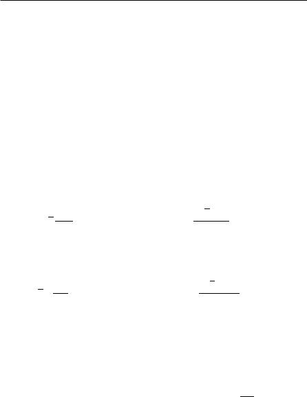
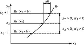
The Prandtl mixing-length theory (1925) is the simplest and the oldest of all turbulence closure models. The mixing length l is the distance a turbulent eddy can travel in a turbulent flow field until it has completely mixed with its surroundings and lost its identity due to the dissipation of its energy. In order to estimate the mixing length, a liquid element with mean velocity ij1(x2) in the main flow direction at the position x2 is regarded, Fig. 3.10. Due to the turbulent fluctuating velocity component u'2, this element may be transported to some position (x2 + l1) or (x2
– l1) below or above the original one. At these new positions, the velocity ij1(x2) of the element differs from the mean velocity ij1 (x2 ρ l1) = ij1 (x2) ρ l1dij1/dx2 of the surroundings by the term
'u |
uc |
r l |
du1 |
, |
(3.105) |
|
|||||
1 |
1 |
1 dx |
|
||
|
|
|
2 |
|
|
which is regarded as fluctuation velocity. Hence, the fluctuation velocity is expressed using the time-averaged velocity again. Due to mass conservation, the fluctuation velocities normal to the mean flow direction must be of the same order:
|
uc |
|
l |
du1 |
, |
|
uc |
|
l |
du1 |
. |
(3.106) |
|
|
|
|
|
||||||||||
|
|
|
|||||||||||
|
1 |
|
1 |
dx |
|
|
2 |
|
2 |
dx |
2 |
|
|
|
|
|
|
2 |
|
|
|
|
|
|
|
|
|
According to Fig. 3.10, where dij1/dx2 > 0, the product u'1u'2 of both velocity fluctuations is always negative. If dij1/dx2 < 0, u'1u'2 > 0. Thus, the signs of both expressions are always different, and the expression for the turbulent stress becomes
|
|
|
U |
|
Ul2 |
|
du1 |
|
|
du1 |
µ |
du1 |
|
|
||
|
|
|
|
ucuc |
, |
(3.107) |
||||||||||
W |
x1 |
,t |
||||||||||||||
dx |
dx |
dx |
||||||||||||||
|
|
1 2 |
|
|
|
|
t |
|
|
|||||||
|
|
|
|
|
|
|
2 |
|
2 |
|
2 |
|
|
|||
3.1 Description of the Continuous Phase |
73 |
|
|
Fig. 3.10. Prandtl mixing-length model
where l2 = l1l2 , and
µ |
Ul2 |
du1 |
(3.108) |
|
|||
t |
dx2 |
|
|
|
|
|
|
is the eddy viscosity. The mixing length l must be determined experimentally. It depends mainly on the distance from a wall. For simple flows, the mixing length model has been shown to produce satisfying results, but this no longer holds true in the case of fully three-dimensional flows. In three-dimensional flows, more detailed models like the two-equation k-e model are used, which introduces two additional differential equations for the description of turbulence.
k-Η Model
The two-equation k-Η model has been published by Launder and Spalding in 1974 [14] and is still the standard turbulence model today. The turbulent viscosity µt has the same dimension as the molecular one: it is the product of velocity and length. Following the approach of Kolmogorov and Prandtl, µt can be expressed as
µt CP U l q , |
(3.109) |
where Cµ is a model constant, and l and q are characteristic length scales and velocities. In the simple mixing length model Cµ·q = l·dij1/dx2 is used, and l is a prescribed function of the distance from a wall. In the model of Launder and Spalding, the characteristic velocity q is taken to be the square root of the turbulent kinetic energy, which is defined by Eq. 3.103. The choice of an expression describing the length scale is much more complicated. The most popular model is based on the fact that in flows where the production of turbulent kinetic energy equals its dissipation, the dissipation rate Η , the length scale l, and the turbulent kinetic energy k can be related by
H | |
k3 / 2 |
|
(3.110) |
|
l . |
||||
|
||||