

Baumgarten
.pdf94 4 Modeling Spray and Mixture Formation
Fig. 4.7. Droplet size distribution: definition of relevant parameters
This problem is usually solved using the method of Lagrange multipliers. The solution is an exponential distribution of the form
Pi exp Ο0 Ο1 f1 di ... Οm fm di , |
(4.29) |
with as many Lagrange multipliers (Ο0,Ο1, Ο2,…Οm) as constraints. To evaluate the Lagrange multipliers, the constraints (Eqs. 4.25 and 4.28) are used. This results in a system of non-linear equations that has to be solved [1]. Further information about the MEF is given, for example, in [128, 25, 2].
The MEF has been used by several authors in order to reconstruct drop size distributions. For example, Dobre and Bolle [28] used the MEF in order to predict the drop size distribution of an ultrasonic atomizer, and Cousin et al. [26] predicted drop size distributions in sprays from pressure-swirl atomizers. Gavaises and Arcoumanis [39] also applied the MEF to hollow-cone sprays and determined the droplet size distribution at every stage of liquid film atomization and, in the case of the subsequent droplet break-up, using only mass conservation and Eq. 4.28 as constraints. Arcoumanis et al. [7] estimated droplets sizes from secondary breakup processes in full-cone diesel sprays. Further applications of the MEF are summarized in [10].
4.1.3 Turbulence-Induced Break-Up
Huh and Gosman [56] have published a phenomenological model of turbulenceinduced atomization for full-cone diesel sprays, which is also used to predict the primary spray cone angle. The authors assume that the turbulent forces within the liquid emerging from the nozzle are the producers of initial surface perturbations, which grow exponentially due to aerodynamic forces and form new droplets. The wavelength of the most unstable surface wave is determined by the turbulent length scale. The turbulent kinetic energy at the nozzle exit is estimated using simple overall mass, momentum, and energy balances.
The atomization model starts with the injection of spherical blobs the diameter of which equal the nozzle hole diameter D. Initial surface waves grow due to the relative velocity between gas and drop (Kelvin-Helmholtz (KH) mechanism) and break up with a characteristic atomization length scale LA and time scale ΩA. The effects of turbulence are introduced by postulating that, on the one hand, the char-

4.1 Primary Break-Up 95
acteristic atomization length scale LA is proportional to the turbulence length scale
Lt,
LA C1Lt C2 Lw , |
(4.30) |
where C1 = 2.0, C2 = 0.5, and Lw is the wavelength of surface perturbations determined by turbulence, and that, on the other hand, the characteristic atomization time scale ΩA is a linear combination of the turbulence time scale Ωt (from nozzle flow) and the wave growth time scale Ωw (KH model),
W A C3Wt C4Ww Wspontaneous Wexp onential , |
(4.31) |
where C3 = 1.2 and C4 = 0.5 [55]. The spontaneous growth time is due to jet turbulence, while the exponential one is caused by the KH wave growth mechanism. The wave growth time scale Ωw provided by the KH instability theory applied to an infinite plane is
ª |
Ul Ug |
|
§Uinj · |
2 |
V |
º 1 |
|
||
Ww « |
|
|
¨ |
|
¸ |
|
|
» |
(4.32) |
Ul Ug |
2 |
Lw |
3 |
||||||
«« |
|
© |
¹ |
|
Ul Ug Lw »» |
|
|||
¬ |
|
|
|
|
|
|
|
¼ |
|
for an inviscid liquid. The turbulent length and time scales Lt0 and Ωt0 at the time the blob leaves the nozzle are related to the average turbulent kinetic energy k0 and the average energy dissipation rate Η at the nozzle exit:
Lt |
Cµ |
k1.5 |
, |
Lt0 |
Cµ |
k01.5 |
(4.33) |
||||
|
H |
H0 |
|
||||||||
Wt |
Cµ |
|
k |
|
, |
Wt0 |
Cµ |
k0 |
|
, |
(4.34) |
|
H |
H0 |
|||||||||
|
|
|
|
|
|
|
|
||||
where Cµ = 0.09 is a constant given in the k-Η-model [71]. In the above equations k0 and Η are estimated as follows [55]:
k0
H0
|
U 2 |
ª |
1 |
|
|
º |
|
|
||||
|
|
inj |
« |
|
Kc 1 |
s2 » |
|
(4.35) |
||||
|
|
|
2 |
|
||||||||
|
8L / D «C |
d |
|
|
» |
|
|
|||||
|
|
|
¬ |
|
|
|
|
¼ |
|
|
||
|
|
U 3 |
ª |
|
1 |
|
|
º |
|
|
||
KH |
inj |
|
« |
|
|
Kc 1 |
s2 » |
, |
(4.36) |
|||
2L |
|
2 |
|
|||||||||
|
|
|
«C |
|
|
» |
|
|
||||
|
|
|
¬ |
|
|
d |
|
|
¼ |
|
|
|
where Cd is the discharge coefficient, KΗ = 0.27 is a model constant, Kc = 0.45 and s = 0.01 are the form loss coefficient and the area ratio at the contraction corner (both values for sharp-edged entry), and L is the nozzle hole length.

96 4 Modeling Spray and Mixture Formation
In order to predict the primary spray cone angle, Huh and Gosman [56] assume that the spray diverges with a radial velocity LA0 /ΩA0. The combination of the radial and axial velocities gives the spray cone angle Ι:
§I · |
LA0 |
/WA0 |
|
|
|||
tan ¨ |
|
¸ |
|
|
. |
(4.37) |
|
2 |
Uinj |
||||||
© |
¹ |
|
|
||||
The direction of the resulting velocity of the primary blob inside the 3D spray cone is randomly chosen, see also Sect. 4.1.1.
From the atomization length and time scales, Eqs. 4.30 and 4.31, the break-up rate of the primary blob and the size of the new secondary drops are derived (new drops are regarded as secondary ones). The break-up rate of a primary blob is set proportional to the atomization length and time scale with an arbitrary constant,
d |
ddrop t k1 |
LA t |
, |
(4.38) |
|
dt |
W A t |
||||
|
|
|
where k1 = 0.05. Analogously to the KH model (Sect. 4.2.4), the primary blob radius is reduced by break-up. The values of the atomization length and time scales in Eq. 4.38 are time-dependent because outside the nozzle the internal turbulence of parent drops decays with time as they travel downstream. Hence, the actual values of turbulent kinetic energy and dissipation must be corrected. Assuming isotropic turbulence and negligible diffusion as well as convection and production of turbulent kinetic energy during this time, the simplified k-Η equations are
|
|
dk t |
H |
|
|
|
(4.39) |
||
|
|
|
|
|
|
||||
|
|
dt |
t |
|
|
|
|||
|
|
|
|
|
|
|
|
||
and |
|
|
|
|
|
|
|||
|
dH t |
H t |
2 |
|
|
||||
|
|
|
|
|
|
|
|
(4.40) |
|
|
dt |
CH |
k t , |
||||||
|
|
||||||||
where CΗ = 1.92. These equations can be solved analytically. Eq. 4.39 can be re-
written as Ηt dt = -dk(t), and Eq. 4.40 gives dΗt /Ηt = -CΗ(Ηt /k(t))dt, which results in
dH t |
C |
dk t |
. |
(4.41) |
|||
H |
|
t |
|
|
|||
H |
k t |
|
|||||
|
|
|
|
|
|
||
With the initial values k0 and Η0 at the time the blobs leave the nozzle, the integration from Η0 to Η and k0 to k gives the time-dependent dissipation rate
H t |
§k |
|
t |
|
·CH |
|
|
H0 ¨ |
|
|
¸ . |
(4.42) |
|||
k0 |
|
||||||
|
© |
|
¹ |
|
|||
Using Eq. 4.41 in Eq. 4.39 yields
|
|
|
|
|
|
|
|
4.1 Primary Break-Up 97 |
|
|
|
|
|
|
|
|
|
|
dk |
|
t |
|
|
H0 |
dt , |
(4.43) |
|
|
|
|
|||||
|
k t CH |
|
||||||
|
|
k0CH |
|
|||||
and integrating from k0 to k and from t0 to t finally gives the time-dependent turbulent kinetic energy of the drop
|
|
|
|
|
|
|
k0CH |
|
1 |
|
|
|||
|
§ |
|
|
|
|
|
|
|
· |
|
|
|
||
k t |
|
|
|
|
|
|
|
CH |
1 |
|
(4.44) |
|||
¨ |
|
|
|
|
|
|
|
|
¸ |
|
. |
|||
H |
0 |
t |
|
C |
|
1 k |
|
|||||||
|
© |
|
|
H |
|
0 ¹ |
|
|
|
|
||||
The values of k(t) and Η(t) are used in Eqs. 4.33 and 4.34 in order to calculate the time-dependent turbulent length and time scales
|
§ |
0.0828 t ·0.457 |
|
||
Lt t |
Lt0 ¨1.0 |
|
¸ |
(4.45) |
|
Ωt0 |
|||||
|
© |
¹ |
|
||
and |
|
|
|
|
|
Ωt t Ωt0 0.0828 t , |
(4.46) |
||||
which again are inputs in Eqs. 4.30 and 4.31 in order to calculate LA(t) and ΩA(t) and to predict the break-up rate of the primary drop, Eq. 4.38. In Eq. 4.32 the actual relative velocity between drop and gas is used instead of Uinj.
The probability density function for the diameter ddrop of the secondary drops is assumed to be proportional to the turbulence energy spectrum [52],
) ddrop ,t |
C |
k / ke t 2 |
|
|
, |
(4.47) |
1 k / ke t 2 |
11 |
/ 6 |
||||
|
|
|
|
|
|
and as inversely proportional to the atomization time scale as follows:
P ddrop ,t C |
) ddrop ,t |
. |
(4.48) |
|
W A ddrop ,t |
||||
|
|
|
The wave number k is the inverse of the droplet diameter ddrop. Further on, ke(t) = 0.75/Lt(t), and the constant C is determined by the normalization condition
³0φ P( d )dddrop 1. |
(4.49) |
Each time the diameter of the primary drop is reduced by break-up, the diameter of the secondary drops is determined using Eq. 4.47.
The model of Huh and Gosman [56] predicts the spray cone angle of steadyflow single-hole experiments reasonably well. However, the effects of cavitation are not included. Instead it is assumed that the turbulence at the nozzle hole exit
98 4 Modeling Spray and Mixture Formation
completely represents the influence of the nozzle characteristics on the primary spray break-up. The use of this model is limited to sprays from non-cavitating turbulent nozzle hole flows.
4.1.4 Cavitation-Induced Break-Up
Arcoumanis et al. [7] have developed a primary break-up model for full-cone diesel sprays that takes cavitation, turbulence, and aerodynamic effects into account. In order to link the spray characteristics with the nozzle hole flow, the authors use a one-dimensional sub-model to estimate input data like effective hole area Aeff, injection velocity Uinj, and turbulent kinetic energy k. The initial droplet diameter is set equal to the effective hole diameter (blob-method), and the first break-up of these blobs is modeled using the Kelvin-Helmholtz mechanism (see Sect. 4.2.4) in the case of aerodynamic-induced break-up, the model of Huh and Gosman [56] for turbulence-induced break-up, and a new phenomenological model in the case of cavitation-induced break-up. This cavitation-induced break-up model will be described in the following. It assumes that the cavitation bubbles are transported to the blob surface by the turbulent velocity inside the liquid and either burst on the surface or collapse before reaching it. For both cases, a characteristic time scale is calculated, and the smaller one causes break-up.
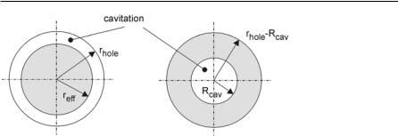
Bubble collapse: in order to estimate the collapse-time, the cavitation bubbles are lumped together into a single big artificial bubble occupying the same area as all the small ones, Fig. 4.8:
Rcav |
rhole2 reff2 , reff |
Aeff / S . |
(4.50) |
Although the collapse-time of cavitation bubbles is directly dependent on their size (smaller bubbles collapse earlier) the radius of this artificial bubble, which is always bigger than the radius of any single bubble present in the nozzle hole flow, is used in order to estimate the atomization time from the Rayleigh theory of bubble dynamics [18]:
Wcoll 0.9145 Rcav |
Ul |
|
Ug ,bubble . |
(4.51) |
Bursting of bubbles: although cavitation structures are usually located along the nozzle hole walls, the artificial bubble is placed in the center of the liquid and then
transported to its surface with a turbulent velocity uturb = (2·k/3)0.5, resulting in a burst time of
Wburst |
rhole Rcav |
. |
(4.52) |
|
|||
|
uturb |
|
|
4.1 Primary Break-Up 99
Fig. 4.8. Estimation of the artificial bubble size
The resulting time scale ΩA of atomization is assumed to be the smaller one of Ωcoll and Ωburst, and the length scale of atomization is given by the correlation
LA 2S rhole Rcav . |
(4.53) |
From LA and ΩA, the force acting on the jet surface at the time of collapsing or bursting of a cavitation bubble with radius Rcav can be estimated from dimensional analysis as
F |
C CN m |
|
|
LA |
, |
(4.54) |
|
|
|||||
total |
|
jet |
|
W A2 |
||
where mjet is the mass of the blob to be atomized, CN = (pback – pvap)/(0.5ΥlU2inj) is the dynamic cavitation number, and C = 0.9 is an empirical constant. The maxi-
mum size of the new droplets is calculated according to the condition Ftotal = Fsurf
with the surface tension force Fsurf = 2Σ rblobς opposing the break-up process. The exact size of the new droplets is sampled from a distribution function. The spray
angle is calculated as proposed in Huh and Gosman (Eq. 4.37):
§I · |
LA /W A |
|
|
|||
tan ¨ |
|
¸ |
|
. |
(4.55) |
|
2 |
Uinj |
|||||
© |
¹ |
|
|
|||
Although the complete aerodynamic, turbulence, and cavitation-induced atomization model of Arcoumanis et al. [7] is quite extensive and takes account of all important effects, the cavitation model is based on strong simplifications. The use of a single artificial bubble for example does not represent the dynamic behavior of a multitude of small bubbles, and the influence of bubble-collapse energy on droplet sizes and spray angle is not included. Although the authors have validated this model against experimental data and have shown its suitability for the simulation of high-pressure diesel injection, the use of a detailed model of bubble dynamics also taking bubble-collapse energy into account would definitely improve the quality of the model.
100 4 Modeling Spray and Mixture Formation
4.1.5 Cavitation and Turbulence-Induced Break-Up
Nishimura and Assanis [91] have presented a cavitation and turbulence-induced primary break-up model for full-cone diesel sprays that takes cavitation bubble collapse energy into account. Discrete cylindrical ligaments with diameter D and volume equal to that of a blob with diameter D are injected, see Fig. 4.9. Each cylinder contains bubbles, according to the volume fraction and size distribution at the hole exit, computed from a phenomenological cavitation model inside the in-
jector. This sub-model also provides the turbulent kinetic energy kflow and the injection velocity Uinj.
The bubbles collapse outside the nozzle, and the energy Ebu = Vbubble pback is re-
leased, resulting in an increase of turbulent kinetic energy kbu = 6Ebu /mcylinder. The reduction of bubble volume V during collapse is calculated using the Rayleigh
theory of bubble dynamics [18]. Assuming isotropic turbulence, the turbulent velocity inside the liquid cylinder can be determined as
uturb |
2 kbu k flow |
. |
(4.56) |
|
3 |
||||
|
|
|
The authors assume that the velocity fluctuations inside the cylinder induce a deformation force
F |
surface dynamic pressure S D |
2 |
D |
Ul |
u2 |
(4.57) |
|
|
|||||
turb |
3 |
|
2 |
turb |
|
|
|
|
|
|
|||
on its surface, and that it breaks up if the sum of Fturb and the aerodynamic drag force Faero = Σ(2/3)D2hole 0.5Υg U2rel is no longer compensated by the surface ten-
sion force Fsurf = ΣDς. In this case, the diameter of the original cylinder is reduced until Fturb + Faero = Fsurf again.
Fig. 4.9 Primary break-up model of Nishimura and Assanis [91]
4.1 Primary Break-Up |
101 |
|
|
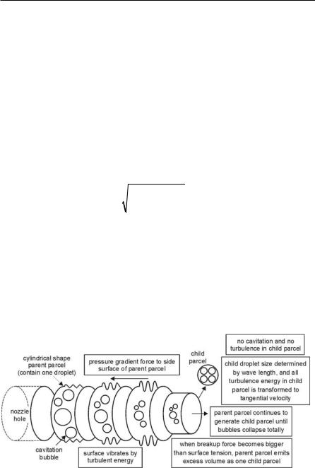
Fig. 4.10 Primary break-up model based on locally resolved break-up rates
The surplus volume (only liquid) forms a parcel of spherical child droplets the diameters of which are estimated by the Kelvin-Helmholtz break-up theory, see Sect. 4.2.4, but uturb is used instead of the relative velocity between gas and liquid in order to predict the surface wave growth. Furthermore, it is assumed that the turbulent kinetic energy contained within the mass of the child droplets is transformed into kinetic energy normal to the original path giving the spray cone angle. The velocity in the original direction is not changed. At the end of bubble collapse, the remaining parent cylinder is transformed into a cylindrical drop and is subject to the secondary aerodynamic-induced break-up like all the child droplets produced before.
The authors have successfully validated their model against experimental data. Because of the detailed modeling of the relevant processes like the increase of break-up energy due to the bubble collapse energy and its direct effect on drop sizes and spray angle, the model is well suited for the simulation of cavitation and turbulence-induced primary break-up. However, it assumes axis-symmetry and is therefore not capable of predicting the influence of asymmetric nozzle hole flows on the 3D structure of primary sprays.
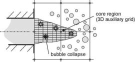
Von Berg et al [143] have published a turbulence and cavitation-induced primary break-up model for full-cone diesel sprays that releases droplets from a coherent core, Fig. 4.10. The sizes and velocity components of the droplets are calculated based on locally resolved turbulence scales and break-up rates on the core surface. The model uses detailed information from a 3D turbulent cavitating nozzle flow simulation as input data. Firstly, this data is utilized in order to estimate the erosion of the jet and the 3D shape of a core region. An auxiliary grid in the core region allows to realize the desired resolution, which cannot be provided by the coarse grid of the combustion chamber. Secondly, a sub-model, based on the simplified Rayleigh theory of cavitation bubble dynamics [18, 143] is used in order to determine the increase of turbulence due to the oscillations of collapsing bubbles within the core. A source term in the k-Η model of each core cell allows to increase the local turbulent kinetic energy and to modify the turbulent time and length scales until the fluid reaches the core surface. Thirdly, an advanced version of the turbulence-induced break-up model of Huh and Gosman [56] is applied locally at the surface elements, which represent the sources of droplet production. The turbulent length scale determines the atomization length scale LA and the droplet size rdrop = LA/2, while the break-up time scale ΩA is a linear combination
102 4 Modeling Spray and Mixture Formation
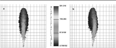
Fig. 4.11. Appearance of spray cone under perpendicular views and droplet velocities. a front view, b side view [143]
of the aerodynamic (Kelvin-Helmholtz-model) and the turbulent time scale. From the local atomization lengths and time scales, the local break-up rates are calculated. The model finally delivers the initial droplet sizes and velocities as well as the initial spray angle.
The model has been successfully validated. In the case of an asymmetric distribution of cavitation within the nozzle hole, the model is able to represent the experimentally observed spray asymmetry: due to better atomization, smaller droplets and an increased spray angle are produced on the cavitation side, Fig. 4.11. The most important features of this primary break-up model are the detailed modeling of the effect of bubble collapse outside the nozzle, the very close linking of nozzle hole flow and spray formation using locally resolved flow properties, and the ability to simulate the influence of asymmetric nozzle flow on the 3D spray structure. This model is well suited for the simulation of high-pressure diesel injection, and because of the very close linking of nozzle hole flow and spray formation, it offers the opportunity to optimize the injection system. However, a complete CFD simulation of the nozzle flow is required as input data.
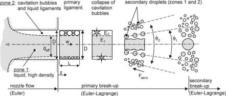
Another detailed cavitation and turbulence-induced primary break-up model for full-cone sprays has been developed by Baumgarten et al. [12, 13, 14]. The model is based on energy and force balances and predicts all starting conditions needed for the simulation of further break-up and mixing processes. The input data is extracted from a CFD calculation of the nozzle flow. This guarantees a very close linking of nozzle characteristics and spray formation. The model simplifies the complex distribution of bubbles and liquid inside the hole and defines two zones (Fig. 4.12): a liquid zone (zone 1) and a mixture zone (zone 2), consisting of liquid and bubbles and surrounding zone 1. The circumferential thickness Lcav (Μ), Fig.
4.13, and the average void fraction 2 = (Υ – Υl)/(Υvap – Υl) of zone 2 as well as further input data like the flow velocity w, the turbulent kinetic energies (k1, k2) and
dissipation rates (Η1, Η2), and the mass flows m1 and m2 of zones 1 and 2 are extracted from a CFD calculation of the nozzle flow. The indices “vap” and “l” indicate vapor and liquid, and Υ is the average density of zone 2.
4.1 Primary Break-Up |
103 |
|
|
Fig. 4.12. Primary break-up model of Baumgarten et al. [13, 14]
The model starts with the injection of cylindrical primary ligaments. Each ligament consists of two zones the distribution of which equals that at the nozzle hole exit. The diameter of the primary ligaments is the hole diameter D, and the length L is equal to the effective diameter deff of the liquid zone.
The size distribution of the cavitation bubbles leaving the nozzle is unknown and must be modeled. Because the stochastic parcel method is used, all bubbles inside a primary ligament have the same size, but from ligament to ligament the sizes differ. The bubble sizes are sampled from a Gaussian distribution (mean value: 10 µm, standard deviation: 10 µm, [13, 14]). The volume of pure vapor and the number of bubbles inside a primary ligament can be calculated from the known average void fraction and size of zone 2. The use of a detailed model of bubble dynamics [13, 14] gives the collapse energy that is released in zone 2 and
the collapse-time tcoll of the bubbles, which is used as the break-up time of the primary ligament. A part of the cavitation energy, Ecav1, is absorbed from zone 1
and contributes to the break-up of this zone. The amount of energy absorbed from zone 1 depends on the distribution of the cavitation zone and is calculated using geometrical relations [13]. Further on, the turbulent kinetic energy produced inside the injection holes is reduced due to dissipation until break-up occurs. The total
break-up energies E1 = Eturb1 + Ecav1 and E2 = Eturb2 + Ecav2 of each zone at the time of break-up are the sums of the particular turbulence and cavitation fractions.
The disintegration of the zones into secondary droplets with a velocity component normal to the spray axis (spray angles Ι1, Ι2, Fig. 4.12) is calculated separately for each zone. The new droplets are exposed to the aerodynamic forces of the secondary break-up.
Break-up of the cavitation zone: It is assumed that the energy E2 is transformed into surface energy Eς2 (formation of n2 new droplets, ς : surface tension fuel/gas) and into kinetic energy Ekin2 normal to the main direction (velocity component vr2 normal to the spray axis),
E |
n VSd 2 |
, |
(4.58) |
|
V 2 |
2 |
2 |
|
|