Baumgarten

84 3 Basic Equations

[9]Jones WP, Launder BE (1972) The Prediction of Laminarization with a Two-Equation Model of Turbulence. Int J Heat and Mass Transfer, vol 15, p 301

[10]Jones WP (1994) Turbulence Modelling and Numerical Solution Methods for Variable Density and Combusting Flows. In Libby PA and Williams FA (editors): Turbulent Reacting Flows. Academic Press, London, pp 309–374

[11]Kays WM, Crawford ME, Weigand B (2005) Convective Heat and Mass Transfer. McGraw-Hill

[12]Kundu PK (1990) Fluid Mechanics. Academic Press

[13]Landau LD, Lifshitz EM (1959) Fluid Mechanics. Addison-Wesley

[14]Launder BE, Spalding DB (1974) The Numerical Computation of Turbulent Flows. Comp Meth Appl Mech Eng 3, pp 269–289

[15]Lettmann H, Eckert P, Baumgarten C, Merker GP (2004) Assessment of Threedimensional In-Cylinder Heat Transfer Models in DI Diesel Engines. 4th European Thermal Sciences Conference, Birmingham

[16]Oertel H, Böhle M (2002) Strömungsmechanik. Second edition, Vieweg-Verlag

[17]Peters N (2000) Turbulent Combustion. Cambridge University Press

[18]Potter MC, Wiggert DC (1997) Mechanics of Fluids. Second Edition, Prentice-Hall Inc

[19]Ramos JI (1989) Internal Combustion Engine Modeling. Hemisphere Publishing Corporation

[20]White FM (1991) Viscous Fluid Flow. McGraw-Hill Inc

[21]Williams FA. (1965) Combustion Theory: Fundamental Theory of Chemically Reacting Flow Systems. Addison-Wesley Publishing Company Inc, Massachusetts

[22]Yakhot V, Orszag SA (1986) Renormalization Group Analysis of Turbulence. I. Basic Theory. Journal of Scientific Computing, vol 1(1), pp 3–51

[23]Yakhot V, Orszag SA (1992) Development of Turbulence Models for Shear Flows by a Double Expansion Technique. Phys Fluids, vol 4(7), pp 1510–1520

86 4 Modeling Spray and Mixture Formation

4.1.1 Blob-Method

The simplest and most popular way of defining the starting conditions of the first droplets at the nozzle hole exit of full-cone diesel sprays is the so-called blobmethod. This approach was developed by Reitz and Diwakar [114, 118]. The blob method is based on the assumption that atomization and drop break-up within the dense spray near the nozzle are indistinguishable processes, and that a detailed simulation can be replaced by the injection of big spherical droplets with uniform size, which are then subject to secondary aerodynamic-induced break-up, see Fig. 4.1. The diameter of these blobs equals the nozzle hole diameter D (mono-disperse injection) and the number of drops injected per unit time is determined from the mass flow rate. Although the blobs break up due to their interaction with the gas, there is a region of large discrete liquid particles near the nozzle, which is conceptually equivalent to a dense core. Assuming slug flow inside the nozzle hole, the conservation of mass gives the injection velocity Uinj (t) of the blobs

where Ahole = ΣD2/4 is the cross-sectional area of the nozzle hole, Υl is the liquid density, and m inj (t) is the fuel mass flow rate (measurement).

If there are no measurements about the injected mass flow, the Bernoulli equation for frictionless flow can be used in order to calculate an upper limit of the initial velocity,

where pinj is the difference between the sac hole and combustion chamber pres-

sures. Because the flow is not frictionless, Uinj,max is reduced by energy losses. According to measurements of Schugger et al. [127], Walther et al. [145], and Mein-

gast et al. [86] the flow velocity at the nozzle hole exit is about 70%–90% of the Bernoulli velocity.

In order to define the velocity components of each blob, the spray cone angle Ι must be known from measurements or has to be estimated using semi-empirical relations (e.g. Hiroyasu and Arai [53]). The direction of the resulting velocity Uinj of the primary blob inside the 3D spray cone is randomly chosen by using two random numbers [1 and [2 in the range of [0, 1] in order to predict the azimuthal angle Μ and the polar angle in the spherical coordinate system, see Fig. 4.2:

88 4 Modeling Spray and Mixture Formation

is the discharge coefficient. By using tabulated inlet loss coefficients (kinlet) and the Blasius or the laminar equation for wall friction, the discharge coefficient is

given by

Assuming a flat velocity profile and using Nurick’s expression for the size of the contraction at the vena contracta [92],

where Cc0 = 0.61. Mass conservation gives the velocity at the smallest flow area:

At the beginning and end of injection, the flow is usually turbulent, the blob size equals the nozzle hole diameter D, and the injection velocity is calculated using Eq. 4.1. During the main injection phase, the flow is usually cavitating, see Fig. 4.3. In this case, the effective cross-sectional area of the nozzle hole exit Aeff

is smaller than the geometrical area Ahole resulting in a decrease of the blob diameter,

while the injection velocity is increased. A momentum balance from the vena contracta (point 1) to the hole exit (point 2), together with the conservation of mass,

Fig. 4.3. One-dimensional cavitating nozzle hole flow

4.1 Primary Break-Up 89

Fig. 4.4. Injection profiles for sharp-edged (SEI) and round-edged inlet (RI), [70]

Fig. 4.5. Dynamic calculation of blob diameter and injection velocity, data from [70]

90 4 Modeling Spray and Mixture Formation

The effective flow area in Eq. 4.12 is

Figures 4.4 and 4.5 show an example of the dynamic calculation of initial blob diameter and injection velocity based on the measured mass flow through a sixhole injector (D = 259 µm) with either a sharp-edged inlet (SEI) or a round-edged inlet (RI). Because of the small mass flows and injection velocities at the beginning and at the end of the injection process, the injection starts and ends with blobs having a diameter equal to D. As soon as cavitation is predicted, the initial diameter decreases rapidly. The highest velocities and the smallest blob diameters are predicted during the main injection process.

Compared to the original blob-method, the dynamic calculation of blob size and injection velocity during the whole injection event introduces the effect of cavitation by decreasing the initial blob size and estimating a more realistic initial velocity. However, only the passive effect of cavitation, the reduction of flow area, is considered. The increase of turbulence and break-up energy due to cavitation bubble implosions is not included.

Altogether, the blob method is a simple and well-known method of treating the primary break-up in Eulerian-Lagrangian CFD codes. As far as there is no detailed information about the composition of the primary spray, and measurements about the spray cone angle are available, it is the best way to define the initial starting conditions for the liquid entering the combustion chamber. Nevertheless, this method does not represent a detailed physical and satisfying modeling of the relevant processes during primary break-up. The most important disadvantage is that the influence of the 3D nozzle hole flow on 3D spray angle and drop size distribution cannot be mapped and that the promotion of primary break-up by turbulence and by implosions of cavitation bubbles outside the nozzle is not regarded at all.

4.1.2 Distribution Functions

This method assumes that the fuel is already fully atomized at the nozzle exit and that the distribution of drop sizes can be described by mathematical functions. In this case, a distribution of droplet sizes is injected. In high-pressure sprays, neither the droplet sizes nor their distribution in the dense spray near the nozzle could be quantified experimentally up to now. Thus the droplet size distribution must be guessed and iteratively adjusted until the measured drop sizes in the far field of the nozzle are similar to the simulated ones. This of course does not represent a detailed modeling of the relevant processes during primary break-up, but can be used as an alternative to the mono-disperse injection of the blob-method.

Full-Cone Sprays

Martinelli et al. [84], for example, assume an initial distribution of drop sizes at the nozzle with the Sauter mean diameter (SMD) given by the correlation

where A2 is independent of the nozzle geometry and of order one. Equation 4.17 accounts for the effect that the initial mean drop size decreases when the chamber pressure increases.

According to Levy et al. [74], the droplet’s diameter D at the nozzle exit should be sampled from a Φ2-law in order to get a good agreement between measured and simulated downstream drop size distributions,

where D SMD / 6 . Further analytical functions to match size distributions in diesel sprays are published in Long et al. [82], Simmons [131], and Levebvre [73].

Hollow-Cone Sprays

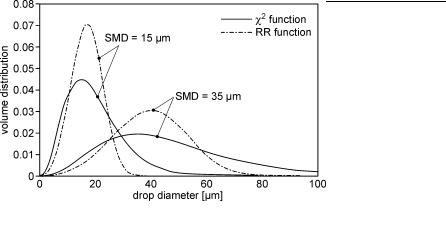
In the case of a hollow-cone spray, an annular liquid sheet is produced at the nozzle orifice forming a free cone-shaped liquid sheet that disintegrates into droplets. The simulation of the liquid phase starts at the point of sheet disintegration, when the first droplets are formed. Two functions are commonly used in order to sample the initial drop sizes, the Φ2 and the Rosin-Rammler distribution. In the case of the Φ2 distribution, the volume distribution (cumulative distribution) V is given by

where V is the fraction of the total volume contained in drops of diameter less than D, and D = SMD/3 is a characteristic mean drop size. The corresponding volume distribution (dV/dD) is shown in Fig. 4.6.

In the case of the Rosin-Rammler distribution, the cumulative volume distribution V is given by

where D is the size of the individual droplets, q is the distribution parameter (q ū 3.5, [49]), and

92 4 Modeling Spray and Mixture Formation

Fig. 4.6. Comparison of the Rosin-Rammler (RR) and Φ2 size distributions [49]

SMD is the Sauter mean diameter of the distribution and is the gamma function:

Figure 4.6 shows a comparison between the Φ2 and the Rosin-Rammler distribution. For a given Sauter mean diameter, the Φ2 distribution yields larger standard deviation and includes more large drops, while the Rosin-Rammler distribution contains more droplets with sizes closer to the SMD value. The larger droplets of the Φ2 distribution will evaporate slower and result in larger tip penetration due to the higher momentum. In the case of pressure-swirl atomizers, the investigations of Han et al. [49] have shown that the measured droplet sizes are better represented by the Rosin-Rammler distribution.

Maximum Entropy Formalism

Instead of defining the shape of the distribution function a priori by mathematical distribution functions, it is possible to predict the function using the so-called Maximum Entropy Formalism (MEF). Due to the use of a physically based criterion, the entropy of the distribution given by Shannon [130], it is possible to estimate the most probable distribution function. For example, if the mean diameter of a spray just after primary break-up is known, either from theoretical calculation or from data extrapolation, and if mass, energy, and momentum have to be conserved (constraints), there is still an infinite number of possible distribution functions that may fit it. Using the Shannon entropy, the one with the largest entropy can be chosen. This distribution is regarded as the most probable one.