

Baumgarten
.pdf44 2 Fundamentals of Mixture Formation in Engines
[14]Gindele J (2001) Untersuchung zur Ladungsbewegung und Gemischbildung im Ottomotor mit Direkteinspritzung. Ph.D. Thesis, University of Karlsruhe, Germany, LogosVerlag, Berlin, ISBN 3-89722-727-4
[15]Gülder ÖL, Smallwood GJ, Snelling DR (1992) Diesel Spray Structure Investigation by Laser Diffraction and Sheet Illumination. SAE paper 920577
[16]Gülder ÖL, Smallwood GJ, Snelling DR (1994) Internal Structure of Transient FullCone Dense Diesel Sprays. Commodia 94, pp 355–360
[17]He L, Ruiz F (1995) Effect of Cavitation on Flow and Turbulence in Plain Orifices for High-Speed Atomization. Atomization and Sprays, vol 5 pp 569–584
[18]Heimgärtner C, Leipertz A (2000) Investigation of Primary Spray Breakup Close to the Nozzle of a Common Rail High Pressure Injection System. Eight International Conference on Liquid Atomization and Spray Systems, Pasadena, CA, USA
[19]Heywood JB (1988) Internal Combustion Engine Fundamentals. McGraw-Hill Book Company
[20]Hiroyasu H, Arai M (1990) Structures of Fuel Sprays in Diesel Engines. SAE-paper 900475
[21]Hiroyasu H, Arai M, Tabata M (1989) Empirical Equations for the Sauter Mean Diameter of a Diesel Spray. SAE paper 890464
[22]Hiroyasu H, Shimizu M, Arai M (1991) Breakup Length of a Liquid Jet and Internal Flow in a Nozzle. ICLASS-91
[23]Hochgreb S, VanDer Wege B (1998) The Effect of Fuel Volatility on Early Spray Development from High Pressure Swirl Injectors. In Direkteinspritzung im Ottomotor, Editor: Spicher U, Expert-Verlag, Rennigen-Malmsheim
[24]Hochgreb S, VanDer Wege B (1999) Investigation of the Effect of Fuel Volatility on Operating Conditions on DISI Sprays. In Direkteinspritzung im Ottomotor II, Editor: Spicher U, Expert-Verlag, Rennigen-Malmsheim
[25]Homburg A (2002) Optische Untersuchungen zur Strahlausbreitung und Gemischbildung beim DI-Benzin-Brennverfahren. Ph.D. Thesis, University of Braunschweig, Germany
[26]Hübel M, Günther H, Ortmann R, Stein J, Yildirim F (2001) Einspritzventile für die Benzin-Direkteinspritzung – ein systematischer Vergleich verschiedener Aktorkonzepte. Wiener Motorensymposium 2001
[27]Hwang SS, Liu Z, Reitz RD (1996) Breakup Mechanisms and Drag Coefficients of High-Speed Vaporizing Liquid Drops. Atomization and Sprays, vol 6, pp 353–376
[28]Iida H, Matsumura E, Tanaka K, Senda J, Fujimoto H, Maly RR (2000) Effect of Internal Flow in a Simulated Diesel Injection Nozzle on Spray Atomization. ICLASS 2000, Pasadena, CA, USA
[29]König G, Blessing M, Krüger C, Michels U, Schwarz V (2002) Analysis of Flow and Cavitation Phenomena in Diesel Injection Nozzles and its Effects on Spray and Mixture Formation. 5. Int Symp für Verbrennungsdiagnistik der AVL Deutschland, BadenBaden
[30]Krzeczkowski SA (1980) Measurement of Liquid Droplet Disintegration Mechanisms. Int J Multiphase Flow, vol 6, pp 227–239
[31]Kuensberg Sarre C, Kong SC, Reitz RD (1999) Modelling the Effects of Injector Nozzle Geometry on Diesel Sprays. SAE paper 1999-01-0912
[32]Lai MC, Yoo JH, Kim SK (1997) High Pressure Gasoline Spray Structure and ist Implications to In-Cylinder Mixture Formation. Tagung Direkteinspritzung im Ottomotor, Haus der Technik, Essen, Germany

References 45
[33]Lefebvre AH (1989) Atomization and Sprays. Hemisphere Publishing Corporation, New York, Washington, Philadelphia, London
[34]Lenz HP (1992) Mixture Formation in Spark-Ignition Engines. Springer-Verlag Wien, New York, ISBN 3-211-82331-X (Springer) and ISBN 1-56091-188-3 (SAE)
[35]Mohammadi A, Kidoguchi Y, Miwa K (2002) Effect of Injection Parameters and Wall-Impingement on Atomization and Gas Entrainment Processes in Diesel Sprays. SAE paper 2002-01-0497
[36]Nayfey AH (1968) Nonlinear Stability of a Liquid Jet. Physics of Fluids, vol 13, no 4, pp 841–847
[37]Ohnesorge W (1931) Die Bildung von Tropfen an Düsen und die Auflösung flüssiger Strahlen. Zeitschrift für angewandte Mathematik und Mechanik, Bd.16, Heft 6, pp 355–358
[38]Ohyama Y, Ohsuga M, Nogi T, Fujieda M Shirashi T (1998) Mixture Formation in Gasoline Direct Injection Engines. In Direkteinspritzung im Ottomotor, Editor: Spicher U, Expert-Verlag, Rennigen-Malmsheim
[39]Potz D, Christ W, Dittus B (2000) Diesel Nozzle – the Determining Interface Between Injection System and Combustion Chamber. THIESEL 2000, pp 249–258
[40]Preussner C, Döring C, Fehler S, Kampmann S (1998) GDI: Interaction Between Mixture Preparation, Combustion System and Injector Performance. SAE paper 980498
[41]Prosperetti A, Lezzi A (1986) Bubble Dynamics in a Compressible Liquid. Part 1. First-Order Theory. J Fluid Mech, vol 168, pp 457–478
[42]Rayleigh Lord FRS (1878) On the Stability of Liquid Jets. Proc. of the Royal Society London
[43]Reitz RD (1978) Atomization and other Breakup Regimes of a Liquid Jet. Ph.D. Thesis, Princeton University
[44]Reitz RD, Bracco FV (1986) Mechanisms of Breakup of Round Liquid Jets. Enzyclopedia of Fluid Mechanics, Gulf Pub, NJ, 3, pp 233–249
[45]Reitz RD, Diwakar R (1987) Structure of High-Pressure Fuel Sprays. SAE paper 870598
[46]Robert Bosch GmbH (1999) Diesel Einspritzsysteme – Unit Injector System / Unit Pump System. Technische Unterrichtung
[47]Robert Bosch GmbH (1999) Diesel-Speichereinspritzsystem Common Rail. ISBN 3- 934584-13-6
[48]Rutland DF Jameson GJ (1970) Theoretical Prediction of the Size of Drops Formed in the Breakup of Capillary Jets. Chem Eng Science, vol 25, p 1689
[49]Schugger C, Renz (2003) Experimental Investigations on the Primary Breakup Zone of High Pressure Diesel Sprays from Multi-Orifice Nozzles. ICLASS 2003
[50]Schugger C, Renz U (2001) Experimental Investigations on the Primary Breakup of High Pressure Diesel Sprays. ILASS-Europe 2001
[51]Soteriou C, Andrews R, Smith M (1995) Direct Injection Diesel Sprays and the Effect of Cavitation and Hydraulic Flip on Atomization. SAER paper 950080
[52]Soteriou C, Andrews R, Torres N, Smith M, Kunkulagunta R (2001) Through the Diesel Nozzle – a Journey of Discovery II. ILASS-Europe 2001, Zürich
[53]Stegemann J, Seebode J, Baltes J, Baumgarten C, Merker GP (2002) Influence of Throttle Effects at the Needle Seat on the Spray Characteristics of a Multihole Injection Nozzle. ILASS-Europe 2002, Zaragoza, Spain
[54]Su TF, Farrell PV, Nagarajan RT (1995) Nozzle Effect on High Pressure Diesel Injection. SAE paper 950083

46 2 Fundamentals of Mixture Formation in Engines
[55]Tamaki N, Shimizu M, Hiroyasu H (2000) Enhanced Atomization of a Liquid Jet by Cavitation in a Nozzle Hole. 8th Int Conf on Liquid Atomization and Spray Systems, Pasadena, CA, USA
[56]Torda TP (1973) Evaporation of Drops and Breakup of Sprays. Astronautica Acta, vol 18, p 383
[57]Urlaub AG, Chmela FG (1974) High-Speed Multifuel Engine: L9204 FMV, SAE paper 740122
[58]van Basshuysen R, Schäfer F (2002) Handbuch Verbrennungsmotor. ISBN 3-528- 03933-7, Vieweg-Verlag, Braunschweig, Wiesbaden
[59]Wierzba A (1993) Deformation and Breakup of Liquid Drops in a Gas Stream at Nearly Critical Weber Numbers. Experiments in Fluids, vol 9, pp 59–64
[60]Wu PK, Faeth GM (1995) Onset and End of Drop Formation along the Surface of Turbulent Liquid Jets in Still Gases. Phys. of Fluids 7 (11)
[61]Youle AJ, Salters DG (1994) A Conductivity Probe Technique for Investigating the Breakup of Diesel Sprays. Atomization and Sprays, vol 4, pp 253–262
[62]Yuen MC (1968) Non-linear Capillary Instability of a Liquid Jet. J Fluid Mech, vol 33, p 151
[63]Zhao FQ, Lai MC, Harrington D (1995) The Spray Characteristics of Automotive Port Fuel Injection – A Critical Review. SAE paper 950506
3 Basic Equations
3.1 Description of the Continuous Phase
3.1.1 Eulerian Description and Material Derivate
In this section, the basic equations for the description of multi-dimensional flow fields will be derived. In internal combustion engines, such flows are the airflow inside the induction system, the gas flow inside the cylinder, and the flow of burnt gases through the exhaust system. The flow of fuel through the three-dimensional injection nozzle geometry is an example of a liquid flow field.
In solid rigid body mechanics, the position in space of a special particle as function of time t is usually the quantity of interest, and from this information all the other questions, such as the amount of velocity and acceleration, may be answered. Hence, all flow quantities F are given as function of particle and time,
F F particle,t , |
(3.1) |
which is called a Lagrangian description. If the vector x = x (particle, t) denotes the position of the particular particle, velocity and acceleration are simply given by u& = d x& (particle, t)/dt and a& = d2 x (particle, t)/dt2. In order to describe the spatial and temporal development of pressure, density, temperature, magnitude, and direction of velocity etc. in a complete flow field using the Lagrangian approach, the position, pressure, density, temperature and velocity of every liquid element inside the flow field have to be calculated. Then, if for example the temporal development of pressure at a fixed point inside the flow field is required, the pressures of the liquid elements that passed this point during the time span of interest have to be listed in the correct order. It is obvious that the Lagrangian approach is well suited for the description of disperse phases (e.g. sprays consisting of liquid droplets), but not for that of continuous fluids.
In a continuum, the flow quantities change continuously in space. In contrast to a dispersed phase, in which the density of the fluid of interest is zero in the volume between two fluid elements, and for which the exact position and size of the elements must be known in order to describe the spatial and temporal distribution of the relevant flow quantities, it is not necessary to distinguish between different fluid elements in the case of a continuum. It is more convenient to describe the flow quantities as a function of a point in space (related to a fixed coordinate system) and time, regardless of what element of liquid happens to be there at any particular time:

48 3 Basic Equations
& |
(3.2) |
F F x,t . |
In order to describe a complete flow field, this approach is applied to all points x& in space. Such a description is called a Eulerian description.
In differential equations, often the time derivate is used. Using the Lagrangian description, the time derivate of F is
dF |
|
particle,t |
|
|
DF |
. |
(3.3) |
|
|
dt |
|
|
Dt |
|
|
This so-called substantial or material derivate describes the complete derivate of the property F of a liquid element. Remember that all flow quantities are only a function of particle and time. In contrast to this, the Eulerian approach describes the flow quantities F as function of point x& = (x1, x2, x3) in space and time t. Us-
ing the chain rule, the quantity dF is
|
dF t,x1 ,x2 ,x3 |
|
wF |
|
dt |
wF |
dx1 |
|
wF |
dx2 |
|
wF |
dx3 . |
|
||||||||||
|
|
wt |
|
wx |
wx |
wx |
|
|
||||||||||||||||
|
|
|
|
|
|
|
|
|
1 |
|
|
|
2 |
|
|
|
3 |
|
|
|
|
|||
The time derivate dF/dt reads |
|
|
|
|
|
|
|
|
|
|
|
|
|
|
|
|
|
|
|
|||||
|
dF t,x1 ,x2 ,x3 |
|
wF dt |
|
wF dx1 |
|
wF dx2 |
|
|
wF |
|
dx3 |
. |
|||||||||||
|
dt |
|
wt |
|
dt |
wx |
|
|
dt |
wx |
|
dt |
|
wx |
|
dt |
||||||||
|
|
|
|
|
|
|
|
|||||||||||||||||
|
|
|
|
|
|
|
|
|
1 |
|
|
|
|
2 |
|
|
|
3 |
|
|
|
|||
(3.4)
(3.5)
In order to emphasize that the material derivate is meant, the expression DF/dt is usually used instead of dF/dt. Because dxi /dt = ui, the material derivate now reads
DF |
|
wF |
u1 |
wF |
u2 |
wF |
u3 |
wF |
, |
(3.6) |
Dt |
|
wt |
wx |
wx |
wx |
|||||
|
|
|
1 |
2 |
3 |
|
|
|||
where u& = (u1, u2, u3) is the velocity vector. The Lagrangian and the Eulerian approaches, if applied to a special problem, must have the same overall result. For example, the resulting acceleration of a liquid element passing any point in space (Lagrangian description) must be identical to the resulting acceleration at this point predicted by the Eulerian approach. In order to explain the different terms in Eq. 3.6, the flow through a converging nozzle shall be regarded. Due to the reduction of cross-sectional area, the flow velocity is larger at an upstream position (point A) than at a downstream position (point B). The first partial derivate on the right hand side of Eq. 3.6 is the local derivate. It describes the temporal change of F at a fixed point in space and is equal to zero at points A and B if the flow is steady. However, the flow velocity at point B is always larger than at point A, and a liquid element passing point A will experience an additional acceleration which is not included in the local derivate. This additional acceleration is expressed by the remaining three terms on the right hand side of Eq. 3.6, the so-called convective derivate. Hence, the Eulerian description enables us to distinguish between a local and a convective part of the material derivate, while the Lagrangian description does not.
3.1 Description of the Continuous Phase |
49 |
|
|
Eq. 3.6 can be expressed in a much shorter form,
DF |
|
wF |
ui |
wF |
, |
(3.7) |
Dt |
|
wt |
wx |
|||
|
|
|
|
i |
|
|
using the so-called index notation (Einstein notation). This convention states that whenever the same index appears twice in a term (here: i), summation over the range of& that index (here: i = 1, 2, 3) is implied.
If F is a vector field, e.g. a velocity field, the equation for every component (coordinate direction j = 1, 2, 3, Cartesian coordinate system) reads
DFj |
|
wFj |
u |
i |
wFj |
, |
(3.8) |
Dt |
|
wt |
wx |
||||
|
|
|
|
||||
|
|
|
|
|
i |
|
|
while the more generalized vector form valid in any coordinate system is
DF& |
|
wF& |
& |
& |
(3.9) |
Dt |
|
wt u |
F . |
||
|
|
||||
3.1.2 Conservation Equations for One-Dimensional Flows
Multi-dimensional flows can often be treated in a simplified manner as onedimensional. Then, the flow quantities only change in the main flow direction. In this case, it is convenient to apply the conservation equation in integral form, which means that the basic fluid equations are applied to a control volume including the complete area of interest. In contrast to this, the conservation equations in differential form are obtained if the basic fluid equations are applied to an infinitesimal elemental volume. The differential equations, which are derived in Sect. 3.1.3, are usually appropriate when the distributive conditions (three-dimensional flow fields) are desired, e.g. the velocity, temperature, and pressure fields inside a combustion chamber. In the following, the integral conservation equations are derived and simplified for one-dimensional flows.
3.1.2.1 Conservation of Mass
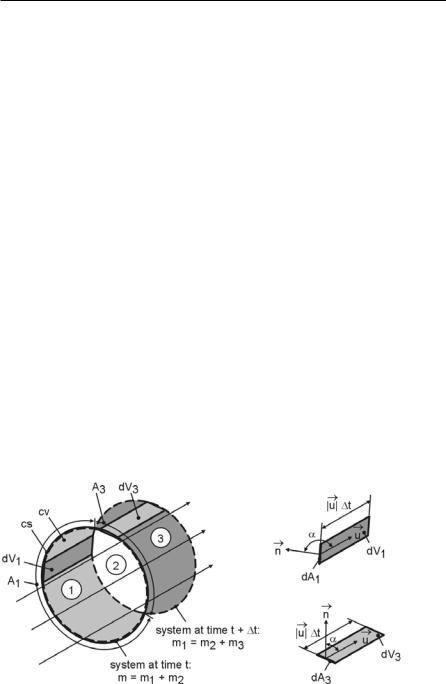
Consider a fixed collection of fluid particles as denoted by the dotted lines in Fig. 3.1. Such a collection of fluid particles (Lagrangian approach) is called a system. The system is shown at times t and t+ t. According to the law stating that mass must be conserved, the mass of the system remains constant:
Dmsys |
0 . |
(3.10) |
|
Dt |
|||
|
|
However, the Eulerian description is usually used in fluid dynamics, and an expression for mass conservation using a control volume that is fixed in space and
50 3 Basic Equations
passed by the flow without resistance must be found. Such a fixed control volume (cv), also shown in Fig. 3.1, equals the volume of the system at time t. Using the masses contained in the volumes 1, 2, and 3 at times t and t + t, the left hand side of Eq. 3.10 becomes
Dmsys |
|
lim |
m3 t 't m2 t 't m2 t m1 t |
|
|||||||
Dt |
|
|
|
|
't |
|
|||||
'to0 |
|
|
|
|
|||||||
|
lim |
m2 t 't m1 t 't m2 t m1 t |
|
|
|||||||
|
|
|
|
|
|
|
|||||
|
'to0 |
|
|
|
't |
|
|||||
|
lim |
m3 t 't m1 t 't |
|
|
|
||||||
|
|
|
|||||||||
|
|
'to0 |
|
't |
|
||||||
|
|
wmcv |
|
+ lim |
m3 t 't m1 t 't |
. |
|
||||
|
|
|
|
(3.11) |
|||||||
|
|
wt |
|
|
'to0 |
't |
|||||
In order to find expressions for the masses m3 (t+ t) and m1 (t+ t) contained in the volumes 1 and 3, the volumes V1 and V3 are needed. These volumes can be calculated from
dV1 |
n& u&'tdA1 and dV3 |
n& u&'tdA3 , |
(3.12) |
||||||||
Fig. 3.1, and the desired expressions can be written as |
|
||||||||||
m3 t 't |
³ U |
|
u& |
|
cosD'tdA3 |
³ Un& u&'tdA3 , |
|
||||
|
|
|
|||||||||
|
A3 |
A3 |
|
||||||||
m1 t 't |
³ U |
|
u& |
|
cosD'tdA1 |
³ Un& u&'tdA1. |
(3.13) |
||||
|
|
||||||||||
|
|
||||||||||
|
A1 |
A1 |
|||||||||
Fig. 3.1. System-to-control-volume transformation: system moving through a control volume, two-dimensional flow and control volume
3.1 Description of the Continuous Phase |
51 |
|
|
Remember that the unit vector n& is normal to the surface element dA and always points out of the control volume (cv). Because A3 plus A1 completely surrounds the control volume (A3 + A1 = cv), Eq. 3.11 is equivalent to
Dmsys |
|
wm |
|
|
& |
& |
w |
|
|
& |
& |
|
||
|
|
cv |
+ |
|
Un |
udA |
|
|
UdV + |
|
Un |
udA . |
(3.14) |
|
Dt |
wt |
³ |
wt ³ |
³ |
||||||||||
|
|
|
|
|
|
|
|
|||||||
|
|
|
cs |
|
|
|
cv |
cs |
|
|
|
|||
The left hand side of this equation describes the rate of change of mass in a Lagrangian frame of reference, while the right hand side represents the respective Eulerian description for a fixed control volume. Hence, Eq. 3.14 is the desired sys- tem-to-control-volume transformation.
A more general expression for such a transformation is given by the Reynolds transport theorem,
D |
Nsys |
w |
& |
& |
|
|
|
|
³KUdV +³KUn |
udA , |
(3.15) |
||
Dt |
wt |
|||||
|
|
|
cv |
cs |
|
|
where Nsys is the extensive quantity (e.g. mass, energy, momentum) and Κ is the intensive property associated with Nsys, the property per unit mass. The time derivate of the first term on the right hand side can be moved inside the integral, since for a fixed control volume the limits on the volume integral are independent of time.
Combining Eqs. 3.10 and 3.14 results in the continuity equation in integral form:
w |
|
|
& |
& |
|
||
|
|
UdV= |
|
Un |
udA . |
(3.16) |
|
wt ³ |
³ |
||||||
|
|
|
|
||||
|
cv |
|
cs |
|
|
|
|
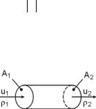
For steady flow, the left hand side is equal to zero. Assuming that the velocity is also normal to all surfaces where fluid crosses (e.g. pipe flow, Fig. 3.2) results in
³ U2u2dA ³ U1u1dA 0 , |
(3.17) |
|
A2 |
A1 |
|
where u&i ui .
If the densities and velocities are uniform over their respective areas, the flow can be treated as one-dimensional, and the continuity equation finally reads
U2u2 A2 U1u1 A1 . |
(3.18) |
Fig. 3.2. Conservation of mass: one-dimensional steady pipe flow
52 3 Basic Equations
3.1.2.2 Conservation of Momentum
Newton’s second law, the momentum equation, states that the sum of all external forces acting on a system equals the rate of change of momentum of the system:
|
|
|
|
DM& |
|
|
¦F& . |
|
(3.19) |
|
|
|
|
|
Dt |
|
|
||||
|
|
|
|
|
|
|
|
|
||
In terms of a control volume, Eq. 3.19 becomes |
|
|
||||||||
|
w |
|
& |
|
|
& |
& |
& |
& |
|
|
|
³ UudV +³ Uu |
n |
u dA |
¦F |
(3.20) |
||||
|
wt |
|||||||||
|
|
cv |
|
cs |
|
|
|
|
|
|
|
|
|
|
|
|
|
& |
|
|
|
by applying Eq. 3.15, where Nsys = |
M = m u& , Κ = u& . The external forces are all |
|||||||||
forces acting on the surfaces of the control volume (pressure, shear, additional surface forces from a solid wall) and body forces (e.g. gravity) acting on the mass inside the control volume.
Eq. 3.20 can be simplified significantly if the control volume has entrances and exits across which the flow quantities may be assumed to be uniform, and if the
flow is steady: |
|
¦N Uu& n& u& A i ¦F& , |
(3.21) |
i 1 |
|
where N is the number of exit and entrance areas. If there is only one entrance and one exit, and if the velocity vector is normal to the entrance and exit areas, the momentum equation reduces to
U2 A2u2u&2 U1 A1u1u&1 ¦F& . |
(3.22) |
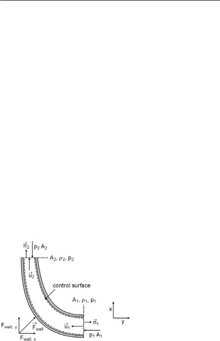
Fig. 3.3. Momentum equation: forces acting on a control volume
3.1 Description of the Continuous Phase |
53 |
|
|
At the entrance u& n& u , since n& and u& point in opposite directions. Note that the momentum equation is a vector equation and consists of one equation for each coordinate direction. If only external forces caused by static pressure and the wall are considered, Fig. 3.3, Eq. 3.22 reads
x direction : |
U A u2 |
F |
p A |
|
||
|
1 1 1 |
wall ,x |
1 1 |
|
||
y direction : |
U |
A u2 |
= F |
p |
A . |
(3.23) |
|
|
2 2 2 |
wall ,y |
|
2 2 |
|
3.1.2.3 Conservation of Energy
Many problems involving fluid motion such as compressible and non-isothermal flows require the use of the energy equation. The energy equation for a system reads
DEt |
|
|
||
|
Q W , |
(3.24) |
||
Dt |
||||
|
|
|
||
where dQ/dt is the amount of heat per unit time and dW/dt is the work per unit time transferred to the system. Et is the total energy consisting of internal energy ΥeV (V: volume of the system, e: internal energy per unit mass), kinetic energy VΥu2/2, and potential energy -VΥ g& x& ( x& : position of system at time t, g& : vector
of gravitational acceleration). In terms of a control volume, Eq. 3.24 becomes
w |
|
|
& |
& |
|
|
|
|
et UdV |
|
Uet u |
ndA Q W |
(3.25) |
wt ³ |
³ |
|||||
|
cv |
|
cs |
|
|
|
by applying Eq. 3.15, where Nsys = Et, Κ = et , and
et |
E |
e |
|
u& |
|
2 |
& |
& |
e |
u2 |
& |
& |
(3.26) |
|
|
||||||||||||
t |
|
|
|
|
g |
x |
|
g |
x . |
||||
|
|
|
|
|
|
|
|
|
|
|
|
|
|
|
m |
|
2 |
|
|
|
2 |
|
|
|
|||
The work-rate term includes the work on the boundaries due to pressure and tangential stresses plus the work added by source terms (e.g. shaft work) minus the reduction due to energy dissipation. The heat-rate term includes the rate-of-energy transfer across the control face due to a temperature difference and the energy production or reduction inside the control volume due to energy sources or sinks such as chemical reactions and radiation.
An important special case of the energy equation occurs in one-dimensional steady flow, see Fig. 3.4. The shear work done at the boundary is zero because the velocity is either zero or normal to the shear force. The work done by pressure,
& |
& |
|
Wp ³ p u |
ndA , |
(3.27) |
cs
is only performed at the inflow and outflow boundaries where the flow velocity is not zero. If dissipation and chemical reactions are neglected, Eq. 3.25 reads