

Baumgarten
.pdf184 4 Modeling Spray and Mixture Formation
Fig. 4.63. Weber numbers of drops before and after impingement, data from [144]
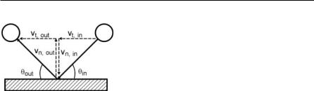
Fig. 4.64. Schematic diagram of the slide model (jet analogy model)
In the slide regime, a droplet striking the wall is given a velocity in the direction of the local tangent to the wall in the manner of a liquid jet. This model is an attempt to develop a simple version of a combined spread/wall film model in analogy to a liquid jet impinging on an inclined wall, Fig. 4.64. It is assumed that the sheet geometry is given by
H H Σ exp Ε 1 /Σ , |
(4.268) |
where the parameter Ε is determined from mass and momentum conservation as
sin |
exp Ε 1 |
|
1 |
. |
(4.269) |
|||
|
|
|
|
|||||
exp Ε 1 |
1 Ε /Σ 2 |
|||||||
|
|
|
|
|||||
In Eq. 4.269, is the jet inclination angle (Fig. 4.64). The probability that an impinging drop slides along the surface at an angle (Fig. 4.64) is assumed to be proportional to the sheet thickness H( ), and is obtained by integrating Eq. 4.268,
|
|
|
4.8 Wall Impingement 185 |
|
|
|
|
|
Σ |
ln 1 p 1 exp Ε , |
(4.270) |
|
|||
|
Ε |
|
|
where p is a random number uniformly distributed in the interval [0, 1].
The most important limitation of the model of Naber and Reitz [90] is that the phenomenon of droplet shattering (splash), which occurs at high impact energy and is important in effecting wall spray dispersion and vaporization, is ignored. This is especially important if the distance between nozzle and wall becomes small. Furthermore, the formation of a liquid film adhering to the wall and its effect on the impingement behavior of drops are not included. Under normal engine conditions, the wall temperatures are below those used in the experiments of Wachters and Westerling [144], and, especially under cold-starting conditions, the transition criterion and the determination of momentum loss during impact are not applicable any more.
Bai and Gosman [11] have developed a more detailed impingement model considering also the splash regime. In the case of a dry wall, the stick and spread regimes are combined and called the adhesion regime, and the stick regime is neglected in the case of a wetted wall because of its typically very low impact energy.
For a dry wall, the transition criterion between adhesion and splash is given as
Adhesion ο Splash |
We |
A La 0.18 , |
(4.271) |
|
crit |
|
|
where the coefficient A is depends on the surface roughness rs, Table 4.6. In the case of an already wetted wall the transition Weber numbers are:
Rebound ο Spread |
Wecrit |
| 5 , |
(4.272) |
Spread ο Splash |
We |
1320 La 0.18 . |
(4.273) |
|
crit |
|
|
In Eq. 4.273 it is assumed that a liquid film can be approximated by a very rough dry wall. Next, the post-impingement characteristics have to be modeled. In the adhesion regime, the incoming droplets are assumed to coalesce to form a local liquid film. In the rebound regime, the droplet bounces off the wall and does not break up, but loses a small part of its kinetic energy by deforming the liquid film. Bai and Gosman [11] use a relationship developed by Matsumoto and Saito [85] for a solid particle bouncing on a solid wall in order to determine the rebound velocity components,
|
|
v |
5 |
v |
, |
|
(4.274 |
|
|
|
|
||||
|
|
t ,out |
7 t ,in |
|
|
|
|
and |
|
|
|
|
|
|
|
Table 4.6. Coefficient A as function of surface roughness rs [11] |
|
||||||
|
|
|
|
|
|
||
rs [µm] |
0.05 |
0.14 |
0.84 |
3.10 |
12.00 |
||
A [/] |
5264 |
4534 |
2634 |
2056 |
1322 |
||
186 4 Modeling Spray and Mixture Formation
Fig. 4.65. Velocity components and respective angles for an impinging drop
vn,out e vn,in , |
(4.275 |
where vt,in and vn,in are the tangential and normal velocity components of the incoming drop, and vt,out and vn,out are the components of the outgoing drop, Fig. 4.65. The quantity e is the restitution coefficient, which is assumed to follow the
relation
e 0.993 1.76 Τin 1.56 Τin2 0.49 Τin3 . |
(4.276) |
In Eq. 4.276, Τin (measured in radians) is the incident angle of the incoming drop, see Fig. 4.65.
In the splash regime, several more post-impingement quantities must be determined. These are the ratio of splashed mass and total incoming mass ms/min, the sizes, velocities, and ejection angles of the new droplets. The mass ratio is modeled by the following relation:
ms |
↑ 0.2 0.6 |
, |
dry wall |
, |
(4.277) |
||||
|
→ |
0.2 |
0.9 |
, |
wetted wall |
|
|||
m |
|||||||||
↓ |
|
|
|
||||||
in |
|
|
|
|
|
|
|||
where is randomly chosen in the interval [0, 1]. Eq. 4.277 corresponds with experimental investigations. In the case of a dry wall there is always some part of liquid lost at the wall, and for the wet wall, the mass ratio is allowed to become larger than 1, because the splashing drops may entrain liquid from the film.
In order to predict the sizes of the new splashed droplets, it is assumed that each incoming droplet parcel produces two new parcels with equal mass ms/ 2, but different drop sizes and velocities. The number of new droplets N = N1 + N2 is de-
termined using a correlation based on experimental results, |
|
|||
N |
5 ♦ |
We |
1÷ . |
(4.278) |
|
♣ |
|
∙ |
|
|
♥ |
We |
≠ |
|
|
crit |
|
||
N1 is randomly chosen in the interval [1, N] and N2 = N – N1. The diameters d1 and d2 of the two new droplet classes are given by mass conservation:
N d3 |
1 |
|
ms |
d3 |
N |
in |
, |
(4.279) |
|
|
|||||||
1 1 |
|
|
|
in |
|
|
||
|
2 min |
|
|
|
|
|||

4.8 Wall Impingement |
187 |
|
|
N2d23 |
1 |
|
ms |
din3 Nin . |
(4.280) |
|
|
||||
|
2 min |
|
|||
The velocity components v&1,out |
|
|
(v1,n ,v1,t ) and v&2,out |
(v2,n ,v2,t ) of the two new |
|
droplet classes are derived from an energy balance. It is assumed that the splashing energy Ek,s
1 |
ms |
|
v&1 |
|
2 |
|
|
v&2 |
|
2 Σς N1d12 N2d22 Ek ,s Ek Ek ,crit , |
(4.281) |
|
|
|
|
||||||||
4 |
|
|
|||||||||
|
|
|
|
|
|
|
|
|
|
|
which consists of kinetic and surface energy, is the difference between the kinetic
energy Ek of the incoming parcel and the critical kinetic energy Ek,crit, below which no splashing occurs. Ek,crit is believed to be lost in deformation, dissipation, and in
producing liquid film energy. Ek,crit is calculated from the critical Weber number:
Ek ,crit |
|
Wecrit |
Σς din2 . |
(4.282) |
|
12 |
|||||
|
|
|
|||
From experimental data on the size-velocity correlation of the new droplets after splashing, the relation
|
|
v& |
|
§ |
d |
· |
§ d |
|
· |
|
||
|
|
|
|
|
||||||||
|
|
&1 |
|
|
| ln ¨ |
1 |
¸ |
/ ln ¨ |
|
2 |
¸ |
(4.283) |
|
|
|
|
|
|
|
||||||
|
|
v2 |
|
|
© din ¹ |
© din ¹ |
|
|||||
is deduced. This relation expresses the observation, that the larger the size of the new droplets, the smaller the magnitude of their velocity. Finally, application of the tangential momentum conservation law yields
ms |
|
v& |
|
cos Τ |
|
ms |
|
|
v& |
|
cos Τ |
2 |
|
c |
m |
|
v& |
|
cos Τ |
in |
. |
(4.284) |
|
|
|
|
|
|
|
||||||||||||||||||
|
|
||||||||||||||||||||||
2 |
|
1 |
|
1 |
2 |
|
|
2 |
|
|
|
|
f in |
|
in |
|
|
|
|
||||
|
|
|
|
|
|
|
|
|
|
|
|
|
|
|
|
|
|
|
|
||||
The wall friction coefficient cf is assumed to be in the range of 0.6 to 0.8, and Τ1 and Τ2 are the ejection angles of the two new parcels. Τ1 is randomly chosen inside an assumed ejection cone (approximately 10°< Τ1 < 160°), and Τ2 is determined from Eq. 4.284. Together with
|
v& |
|
2 |
v2 |
v2 |
and |
|
v& |
|
2 |
v2 |
v2 |
(4.285) |
|
|
|
|
||||||||||
|
1 |
|
|
1,n |
1,t |
|
|
2 |
|
|
2,n |
2,t |
|
the above set of equations can be solved in order to calculate the normal and tangential velocity components of the two new parcels.
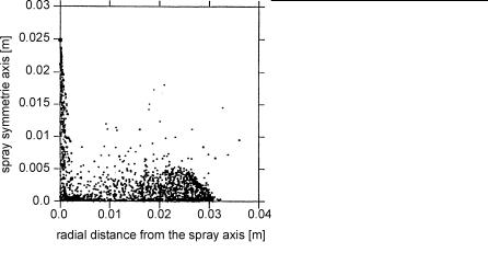
The model of Bai and Gosman [11] has been successfully validated against experimental data. A typical spray pattern (side view, half spray) simulated with this model and showing all the characteristic features of a wall spray is given in Fig. 4.66. The computational parcels are shown as black points.
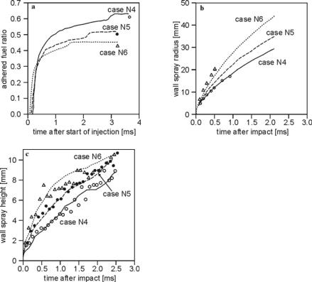
Fig. 4.67 shows comparisons between predicted and measured adhered fuel ratio on the wall, wall spray radius, and wall spray height. Comparisons of local droplet diameters are not given. The experiments were performed by Saito et al. [123], and the boundary conditions are given in Table 4.7.
188 4 Modeling Spray and Mixture Formation
Fig. 4.66. Simulation of an impinging spray [11], t = 2 ms after SOI, atmospheric conditions
Table 4.7. Boundary conditions for the experiments of Saito et al. [123]
Case No |
|
N4 |
N5 |
N6 |
Wall distance [mm] |
25 |
25 |
25 |
|
Gas pressure [MPa] |
0.2 |
0.2 |
0.2 |
|
Gas temperature [K] |
293 |
293 |
293 |
|
Nozzle |
Diameter |
0.25 |
0.25 |
0.25 |
[mm] |
|
|
|
|
Injection |
duration |
2.85 |
2.1 |
1.425 |
[ms] |
|
|
|
|
Injection |
angle |
90 |
90 |
90 |
[deg.] |
|
|
|
|
Injected |
fuel |
35 |
35 |
35 |
[mm3/pulse] |
|
|
|
|
Fuel |
|
diesel |
diesel |
diesel |
Injection |
pressure |
30 |
55 |
120 |
[MPa] |
|
|
|
|
Measurement and simulation agree well. The cusp in the curves of Fig. 4.67a corresponds to the end of injection. After the end of injection, the adhered fuel ratio, which is defined as total mass deposited on the wall divided by the total mass injected at that time, increases, because the deposited mass continues to increase for a short time while the injected mass remains constant. The predictions of wall spray radius (Fig. 4.67b) and wall spray height (Fig. 4.67c) capture the trend that an increase of injection pressure results in larger values of wall spray radius and height. The droplets in the wall spray get larger tangential velocities due to the increased gas velocities along the wall, and larger normal velocities because of a more intense splashing.
4.8 Wall Impingement |
189 |
|
|
Fig. 4.67. a Measured and predicted adhered fuel ratio, b wall spray radius, c wall spray height, [11]
Other detailed wall-impingement models have been developed by O’Rourke and Amsden [95], Lee and Ryou [72], and Stanton and Rutland [132]. Differences between these models and that of Bai and Gosman [11] appear mainly in the splash regime.
In the model of O’Rourke and Amsden [95], the film momentum equation is used in combination with experimental results from Mundo et al. [89] in order to derive the spread-splash transition criterion
E2 |
Υl vn2,in din |
|
ª |
|
§ h |
|
· |
|
Γ |
bl |
º 1 |
|
2 |
E2 |
|
|
||
|
|
« |
min |
¨ |
|
0 |
,1 |
¸ |
|
|
» |
! 57.7 |
|
, |
(4.286) |
|||
|
|
|
|
|
|
|||||||||||||
|
ς |
|
|
d |
|
|
|
d |
|
|
|
crit |
|
|
||||
|
|
« |
|
© |
in |
|
¹ |
|
|
» |
|
|
|
|
|
|||
|
|
|
¬ |
|
|
|
|
|
in ¼ |
|
|
|
|
|
||||
where
190 4 Modeling Spray and Mixture Formation
E |
|
vn,in |
|
|
ς h0 |
|
|
1 |
(4.287) |
||
|
din |
Υl |
|
is the splash Mach number, h0 is the initial film thickness before impact, and Γbl = din /Re)1/2 is a boundary layer thickness. The ratio of splashed mass and incident mass is modeled on the basis of the experimental data of Yarin and Weiss [147],
m |
1.8 104 |
|
E2 |
E2 |
for E2 |
|
E2 7500½ |
|
|||
° |
|
|
crit |
crit |
|
|
|
° |
|
||
s |
® |
|
|
|
|
|
|
|
|
¾ . |
(4.288) |
m |
|
|
|
|
|
|
2 |
|
|||
° |
0.75 |
|
|
|
for |
E |
! 7500 |
° |
|
||
|
¯ |
|
|
|
|
¿ |
|
||||
The prediction of drop radius r is based on the experimental results of Yarin and Weiss [147] and Mundo et al. [89], and is sampled from a truncated NukiyamaTanasawa distribution
|
4 |
|
r |
2 |
ª |
§ |
r |
· |
2 º |
|
|
§ |
2 |
|
|
6.4 |
|
· |
|
f r |
|
|
exp « |
» , |
r |
r |
max ¨ |
Ecrit |
, |
, 0.06 |
¸. |
(4.289) |
|||||||
Σ |
|
r3 |
|
¨ r |
¸ |
|
We |
||||||||||||
|
|
|
« |
» |
max |
in |
¨ |
E2 |
|
¸ |
|
||||||||
|
|
|
max |
¬ |
© |
max ¹ |
¼ |
|
|
© |
|
|
|
|
|
¹ |
|
||
In order to predict the velocity components of the new droplets, O’Rourke and Amsden [95] approximated the velocity distributions reported in [89] and [147]:
v& vc |
n& 0.12 v |
vc |
cos e& sin e& |
p |
0.8v |
|
e& , |
(4.290) |
|
n,out |
n,in |
t,out |
t |
|
t,in |
t |
|
||
where n& is the unit vector normal to the wall surface, e&t |
is the unit vector tangential |
||||||||
to the surface in the plane of |
& |
& |
|
& |
& |
χ |
|
χ |
|
n and the incident drop, ep n |
υ et , vn,out and |
vt ,out are |
|||||||
the normal and tangential velocity fluctuations, and < is the angle that the fluctu-
ating velocity makes with the vector et in the plane of the wall, see Fig. 4.64. The
quantities vχ , vχ , and < are random variables chosen from the following dis-
n,out t,out
tributions:
|
|
|
4 |
|
vc |
2 |
|
ª |
§ vc |
|
· |
2 º |
|
|
|
|
|
|
|||||
f vc |
|
|
|
n,out |
|
|
|
exp « |
¨ |
|
n,out |
¸ |
» (Nukiyama-Tanasawa), |
(4.291) |
|||||||||
|
|
|
|
|
3 |
|
|
|
|||||||||||||||
n,out |
|
|
Σ |
|
0.2v |
|
|
« |
|
¨ |
|
|
|
¸ |
» |
|
|
|
|
|
|
||
|
|
|
|
|
|
|
© |
0.2vn,in ¹ |
|
|
|
|
|
|
|||||||||
|
|
|
|
|
n,in |
|
|
¬ |
|
|
|
|
|
|
¼ |
|
|
|
|
|
|
||
|
|
|
|
1 |
|
|
|
|
|
ª |
|
§ |
|
vtc,out |
|
· |
2 |
º |
|
|
|||
|
|
|
|
|
|
|
|
exp « |
|
|
|
|
» |
|
|
||||||||
f vc |
|
|
|
|
|
|
|
¨ |
|
|
¸ |
|
(Gaussian dist.), |
(4.292) |
|||||||||
|
|
|
|
|
|
|
2 |
|
|
|
|
2 |
|
» |
|||||||||
t,out |
|
|
2Σ 0.1 v |
|
|
|
|
« |
|
¨ |
2 |
0.1 vn,in |
¸ |
|
|
|
|||||||
|
|
|
|
|
|
|
« |
|
¨ |
|
¸ |
|
» |
|
|
||||||||
|
|
|
|
|
n,in |
|
|
|
¬ |
|
© |
|
|
|
|
|
¹ |
|
¼ |
|
|
||
and the angle < is chosen as suggested in the model of Naber and Reitz.
A further wall impingement model has been developed by Lee and Ryou [72]. The main difference to the model of Bai and Gosman [11] is a modified calculation of the dissipated energy due to the impact of a drop on the wetted surface, and the subsequent calculation of the total velocity from the energy conservation law.
4.8 Wall Impingement |
191 |
|
|
Furthermore, the spread-splash transition criterion is determined by using an empirical correlation based on the experimental results of Mundo et al. [89], and only one instead of two new parcels is created in the splash regime. The size and number of the splashed new droplets are determined from the conservation of mass and from experimental data.
4.8.3 Wall Film Modeling
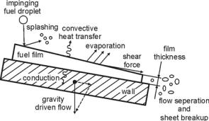
A detailed modeling of wall film evolution includes the simulation of all effects increasing or decreasing the liquid mass on the surface of a wall cell like deposition of droplets, evaporation and film movement, see Fig. 4.68. Film movement can be due to the gravity force or due to exchange of momentum between gas and film or between incident droplets and film. Different classes of wall film models exist. One method is to set up and solve the governing equations for wall films. The other method is to simplify the treatment and to use empirical correlations for the relevant effects.
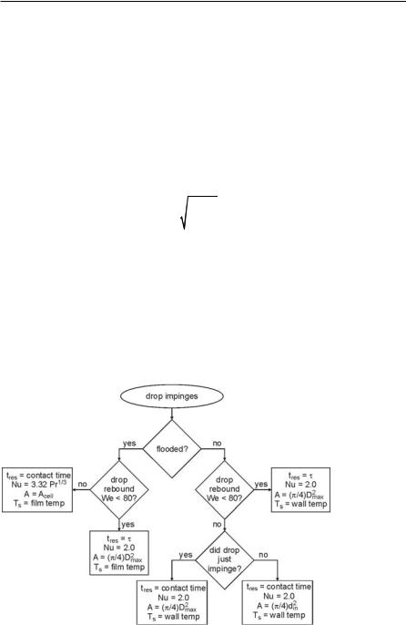
An early model for the simulation of wall film evolution and heat transfer from the wall to the film or to the impinging drops was developed by Eckhause and Reitz [31]. This model includes the impingement model of Naber and Reitz [90], Sect. 4.8.2. The model distinguishes between a flooded (a wall film is present) and a non-flooded case (no wall film), see Fig. 4.69. According to the model of Naber and Reitz [90], only droplets with Wein > 80 (slide) contribute to the formation of a liquid film. The film thickness Γ is calculated separately for each surface cell by taking the total mass of fuel on the surface of a wall cell and dividing by the fuel
density Υl and the wall cell area Acell. The transition criterion between the nonflooded and the flooded case is given as Γ = 2 µm. The total heat transferred to a film or a drop is
Fig. 4.68. The major physical phenomena governing film flow [133]
192 4 Modeling Spray and Mixture Formation
Q A D Ts T tres Qg , |
(4.293) |
where A is the contact area, is the convective heat transfer coefficient (Nu = ( ·Γ)/Ο, Nu: Nusselt number, Γ: film thickness or drop diameter, Ο: thermal conductivity), T is the liquid drop or film temperature, Ts is the surface temperature,
tres is the residence time of the liquid on the surface, and Qg is added in case of wall film formation and is the heat transferred from the gas to the film.
Droplets may either impinge on a dry wall (non-flooded case) or on a liquid wall film (flooded case). Furthermore, droplets may rebound or slide in both cases.
In the case of rebound, the residence time of a drop is assumed to be the first-
order vibration period of an oscillating drop [144], |
|
|||||
tres |
S |
|
Ul din3 |
, |
(4.294) |
|
4 |
V |
|||||
|
|
|
|
|||
and the contact area between the deformed drop and the wall or the film is predicted based on the spreading equation of Akao et al. [3]:
A |
S |
D2 |
, |
D |
0.613 d |
in |
We0.39 . |
(4.295) |
|
||||||||
|
4 |
max |
|
max |
|
in |
|
|
|
|
|
|
|
|
|
|
The surface temperature Ts is the film temperature or the wall temperature, depending on whether a wall film is present or not. The Nusselt number is taken to be Nu = 2.0 for individual droplets.
Fig. 4.69. Heat transfer model of Eckhause and Reitz [31]
4.8 Wall Impingement |
193 |
|
|
For the case of slide, Eckhause and Reitz [31] distinguish between the flooded and the non-flooded regime. In the non-flooded regime the contact area is calculated according to Eq. 4.295 during the time step of first contact, and then the area is A = (Σ4) din2 during the time the droplet slides along the wall. Again, Nu = 2.0 is used and the corresponding surface temperature is the wall temperature. In the flooded regime the droplet becomes part of the wall film. The film temperature is the mass average temperature of all droplets belonging to the film, and the contact
area A is equal to the surface area Acell of the respective wall cell. The gas-phase heat transfer is calculated based on the modified law of the wall (Reitz [116]),
while the liquid-phase heat transfer is based on the heat transfer correlation Nu = 3.32·Pr1/3 for the boundary layer flow.
The temperature change of a film element or a drop is given by
'T |
Q |
, |
(4.296) |
|
m cv,l |
||||
|
|
|
where cv,l is its specific heat capacity and m is the liquid mass of the fuel on a wall cell (flooded case) or the one of a single drop (non-flooded case and rebound).
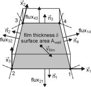
A much more detailed wall film model, which simulates thin fuel film flow on solid surfaces of arbitrary configuration, is presented in Stanton and Rutland [132, 133]. The major mechanical and physical processes like mass, momentum, and pressure contributions to the film due to spray impingement and splashing effects as well as the effects of shear forces, piston acceleration, and gravity are included. The following assumptions are used in the formulation of the model: First, the liquid film is treated as a thin film and the momentum and continuity equations are integrated across the film thickness x&3, see Fig. 4.70. Thus, a two dimensional film is regarded that flows over a three dimensional surface. Fig. 4.70 shows the local coordinate system used for the description of a wall film cell.
Fig. 4.70. Wall film cell and local coordinate system of the film model