- •4.1. Introduction
- •4.2. Areas under continuous probability density functions
- •4.3. The normal distribution
- •1. The total area under the curve is 1.0.
- •4.3.1. Cumulative distribution function of the
- •4.4. The standard normal distribution
- •4.5. Standardizing a normal distribution
- •4.6. The normal distribution approximation to the binomial
- •4.7. The exponential probability distribution
Chapter 4
Continuous random variables and their probability distributions
4.1. Introduction
U p
to this point, we have limited our discussion to probability
distributions of discrete random variables. Recall that a discrete
random variable takes on only some isolated values, usually integers
representing a count. We now turn our attention to the probability
distribution of a continuous random variable- one that can ideally
assume any value in an interval. Variables measured on an underlying
continuous scale, such as weight, strength, life length, and
temperature, have this feature.
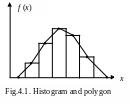
Figure 4.1 displays the histogram and
polygon for some continuous data set.
The smoothed polygon is an approximation
of the probability distribution curve of the continuous random variable X. The probability distribution curve of a continuous random variable is also called
its probability density function.
The
probability density function, denoted by
![]() possesses
the following characteristics:
possesses
the following characteristics:
1.
![]() for all x.
for all x.
2 .
The area under the probability density function
over
all possible values of the random variable X
is equal to 1.
3. Let
a
and b
be two possible values of the random variable X,
with![]() .
Then the probability that X
lies between a
and b
is the area under the density function between a
and b.(Fig.4.2)
.
Then the probability that X
lies between a
and b
is the area under the density function between a
and b.(Fig.4.2)
4.
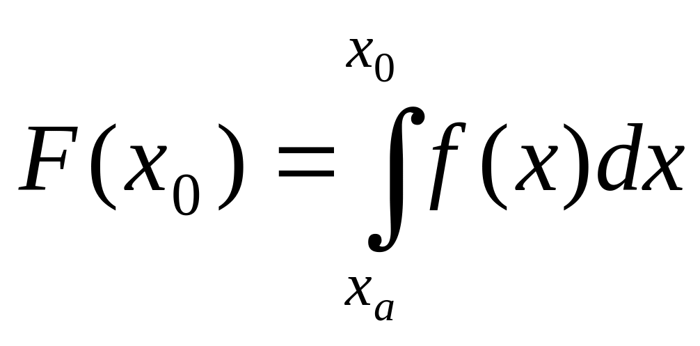
The cumulative distribution function
![]() is the area under the probability density function
up to
is the area under the probability density function
up to
![]()

where
![]() is
the minimum value of the random variable X.
is
the minimum value of the random variable X.
4.2. Areas under continuous probability density functions
Let X
be a continuous random variable with probability density function
and
cumulative distribution function![]() .
Then:
.
Then:
1. The total area under the curve is 1.
2. The area under the curve to the left of is ,
where is any value that the random variable X can take.
T he
area under the probability distribution curve of a continuous random
variable between any two points is between 0 and 1, as shown in
Figure 4.3.
The total area under the probability distribution curve of a continuous random variable is always 1.0 or 100% as shown in Figure 4.4.
Remark:
The probability that a continuous random variable x assumes a single value is always zero.
This is because the area of a line, which represents a single point,
is zero. (Fig.4.5)
In general, if a and b are two of the values that X can assume, then,
![]() and
and
![]() .
.

When
determining the probability of an interval a
to b,
we need not be concerned if either or both end points are included in
the interval. Since the probabilities of
![]() and
and
![]() are
both equal to 0,
are
both equal to 0,
![]() .
.
Exercises
1. Which of the functions sketched in a-d could be a probability density function for a continuous random variable? Why or why not?

f
(x)

1

2
x


0
b)


2. Determine the following probabilities from the curve diagrammed in exercise 1(a).
a)
![]() b)
b)![]()
c)
![]() d)
d)![]()
3.
For the curve
graphed in exercise 1(c) which of the two intervals
![]() or
or
![]() is
assigned a higher probability?
is
assigned a higher probability?
4. The time it takes for a TV repair master to finish his job (in hours) has a
density function of the form
![]()
a) Determine the constant c.
b) What is
the probability that a TV repair master will finish the job in less
than 75 minutes? Between
![]() and
2 hours?
and
2 hours?
5. Suppose that the loss in a certain investment, in thousands of dollars, is a continuous random variable X that has a density function of the form
![]()
a) Calculate the value of k.
b) Find the probability that the loss is at most $500.
6. Let the random variable X has probability density function
![]()
a) Draw the probability density function
b) Show that the density function has the properties of a proper probability density function
c) Find the probability that X takes a value between 0.5 and 1.5.
Answers
2. a) 0.25; b) 0.25; c) 0.25; d) 0; 3. The interval 1.5 to 2 has higher probability; 4. a) -6; b) 5/32 ; 1/2; 5. a) -1/2; b) 3/16; 6. c) 0.75.
