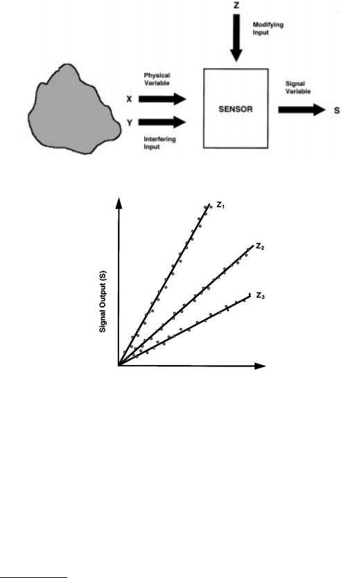
FIGURE 1.4 Interfering inputs.

FIGURE 1.5 Illustration of the effect of a modifying input on a calibration curve.

with Y interfering with the intended measurand X. An example of an interfering input would be a structural vibration within a force measurement system.

Modifying inputs changes the behavior of the sensor or measurement system, thereby modifying the input/output relationship and calibration of the device. This is shown schematically in Figure 1.5. For various values of Z in Figure 1.5, the slope of the calibration curve changes. Consequently, changing Z will result in a change of the apparent measurement even if the physical input variable X remains constant. A common example of a modifying input is temperature; it is for this reason that many devices are calibrated at specified temperatures.

Accuracy and Error

The accuracy of an instrument is defined as the difference between the true value of the measurand and the measured value indicated by the instrument. Typically, the true value is defined in reference to some absolute or agreed upon standard. For any particular measurement there will be some error due to

© 1999 by CRC Press LLC

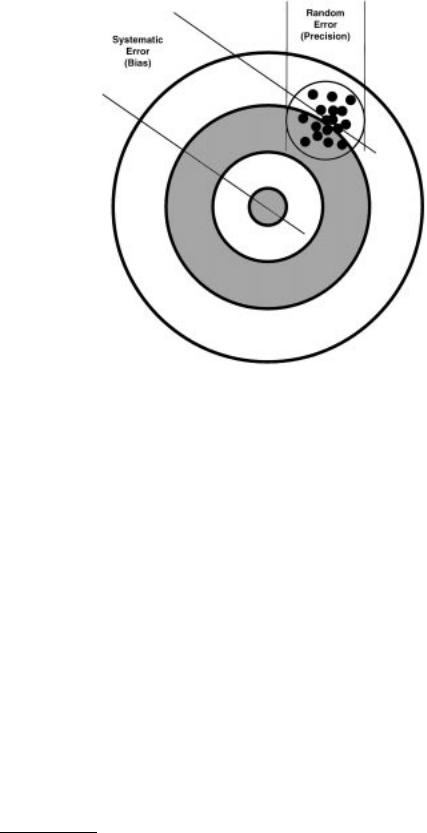
FIGURE 1.6 Target analogy of measurement accuracy.

systematic (bias) and random (noise) error sources. The combination of systematic and random error can be visualized by considering the analogy of the target shown in Figure 1.6. The total error in each shot results from both systematic and random errors. The systematic (bias) error results in the grouping of shots being offset from the bulls eye (presumably a misalignment of the gunsight or wind). The size of the grouping is determined by random error sources and is a measure of the precision of the shooting.

Systematic Error Sources (Bias)

There are a variety of factors that can result in systematic measurement errors. One class of cause factors are those that change the input–output response of a sensor resulting in miscalibration. The modifying inputs and interfering inputs discussed above can result in sensor miscalibration. For example, if temperature is a modifying input, using the sensor at a temperature other than the calibrated temperature will result in a systematic error. In many cases, if the systematic error source is known, it can be corrected for by the use of compensation methods.

There are other factors that can also cause a change in sensor calibration resulting in systematic errors. In some sensors, aging of the components will change the sensor response and hence the calibration. Damage or abuse of the sensor can also change the calibration. In order to prevent these systematic errors, sensors should be periodically recalibrated.

Systematic errors can also be introduced if the measurement process itself changes the intended measurand. This issue, defined as invasiveness, is a key concern in many measurement problems. Interaction between measurement and measurement device is always present; however, in many cases, it can be reduced to an insignificant level. For example, in electronic systems, the energy drain of a measuring device can be made negligible by making the input impedance very high. An extreme example of invasiveness would be to use a large warm thermometer to measure the temperature of a small volume of cold fluid. Heat would be transferred from the thermometer and would warm the fluid, resulting in an inaccurate measurement.

© 1999 by CRC Press LLC

FIGURE 1.7 Example of a Gaussian distribution.

Systematic errors can also be introduced in the signal path of the measurement process shown in Figure 1.3. If the signal is modified in some way, the indicated measurement will be different from the sensed value. In physical signal paths such as mechanical systems that transmit force or displacement, friction can modify the propagation of the signal. In electrical circuits, resistance or attenuation can also modify the signal, resulting in a systematic error.

Finally, systematic errors or bias can be introduced by human observers when reading the measurement. A common example of observer bias error is parallax error. This is the error that results when an observer reads a dial from a non-normal angle. Because the indicating needle is above the dial face, the apparent reading will be shifted from the correct value.

Random Error Sources (Noise)

If systematic errors can be removed from a measurement, some error will remain due to the random error sources that define the precision of the measurement. Random error is sometimes referred to as noise, which is defined as a signal that carries no useful information. If a measurement with true random error is repeated a large number of times, it will exhibit a Gaussian distribution, as demonstrated in the example in Figure 1.7 by plotting the number of times values within specific ranges are measured. The Gaussian distribution is centered on the true value (presuming no systematic errors), so the mean or average of all the measurements will yield a good estimate of the true value.

The precision of the measurement is normally quantified by the standard deviation (σ) that indicates the width of the Gaussian distribution. Given a large number of measurements, a total of 68% of the measurements will fall within ±1σ of the mean; 95% will fall within ±2σ; and 99.7% will fall within

±3σ. The smaller the standard deviation, the more precise the measurement. For many applications, it is common to refer to the 2σ value when reporting the precision of a measurement. However, for some applications such as navigation, it is common to report the 3σ value, which defines the limit of likely uncertainty in the measurement.

There are a variety of sources of randomness that can degrade the precision of the measurement — starting with the repeatability of the measurand itself. For example, if the height of a rough surface is to be measured, the measured value will depend on the exact location at which the measurement is taken. Repeated measurements will reflect the randomness of the surface roughness.

© 1999 by CRC Press LLC