


Leap seconds occur slightly less than once per year because UT1 is currently changing by about 800 ms per year with respect to UTC. The first leap second was introduced on June 30, 1972. So far, all leap seconds have been positive, which indicates that the mean solar second (defined by the Earth’s rotation) is longer than the atomic second (defined by cesium). UTC is running faster than UT1 for two reasons. The first, and most important reason, is that the definition of the atomic second caused it to be slightly shorter than the mean solar second. The second reason is that the speed of the Earth’s rotation is generally decreasing. When a positive leap second is added to UTC, the sequence of events is:
23 h 59 m 59 s
23 h 59 m 60 s
0 h 0 m 0 s
The insertion of the leap second creates a minute that is 61 s long. This effectively “stops” the UTC time scale for 1 s, so that UT1 has a chance to catch up. Unless a dramatic, unforeseen change in the Earth’s rotation rate takes place, future leap seconds will continue to be positive [10, 11].
18.5 Introduction to Time Transfer
Many applications require different clocks at different locations to be set to the same time (synchronization), or to run at the same rate (syntonization). A common application is to transfer time from one location and synchronize a clock at another location. This requires a 1 pulse per second (pps) output referenced to UTC. Once we have an on-time pulse, we know the arrival time of each second and can syntonize a local clock by making it run at the same rate. However, we still must know the time-of-day before we can synchronize the clock. For example, is it 12:31:38 or 12:31:48? To get the time-of-day, we need a time code referenced to UTC. A time code provides the UTC hour, minute, and second, and often provides date information like month, day, and year.
To summarize, synchronization requires two things: an on-time pulse and a time code. Many time transfer signals meet both requirements. These signals originate from a UTC clock referenced to one or more cesium oscillators. The time signal from this clock is then distributed (or transferred) to users.
Time can be transferred through many different mediums, including coaxial cables, optical fibers, radio signals (at numerous places in the spectrum), telephone lines, and computer networks. Before discussing the available time transfer signals, the methods used to transfer time are examined.
Time Transfer Methods
The single largest contributor to time transfer uncertainty is path delay, or the delay introduced as the signal travels from the transmitter (source) to the receiver (destination). To illustrate the path delay problem, consider a time signal broadcast from a radio station. Assume that the time signal is nearly perfect at its source, with an uncertainty of ±100 ns of UTC. If a receiving site is set up 1000 km away, we need to calculate how long it takes for the signal to get to the site. Radio signals travel at the speed of light ( 3.3 s km–1). Therefore, by the time the signal gets to the site, it is already 3.3 ms late. We can compensate for this path delay by making a 3.3 ms adjustment to the clock. This is called calibrating the path.
There is always a limit to how well we can calibrate a path. For example, to find the path length, we need coordinates for both the receiver and transmitter, and software to calculate the delay. Even then, we are assuming that the signal took the shortest path between the transmitter and receiver. Of course, this is not true. Radio signals can bounce between the Earth and ionosphere, and travel much further than the distance between antennae. A good path delay estimate requires knowledge of the variables that influence radio propagation: the time of year, the time of day, the position of the sun, the solar index, etc. Even then, path delay estimates are so inexact that it might be difficult to recover time with ±1 ms uncertainty (10,000 times worse than the transmitted time) [12, 13].
© 1999 by CRC Press LLC
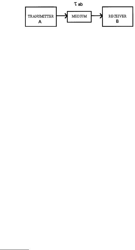
FIGURE 18.1 One-way time transfer.
Designers of time transfer systems have developed many innovative ways to deal with the problem of path delay. The more sophisticated methods have a self-calibrating path that automatically compensates for path delay. The various time transfer systems can be divided into five general categories:
1.One-way method (user calibrates path): This is the simplest and most common kind of time transfer
system, a one-way system where the user is responsible for calibrating the path (if required). As
illustrated in Figure 18.1, the signal from the transmitter to the receiver is delayed τab by the medium. To obtain the best results, the user must estimate τab and calibrate the path by compensating for the delay.
Often, the user of a one-way system only requires timing uncertainty of ±1 s, so no effort is made to calibrate the path. For example, the user of a high-frequency (HF) broadcast can synchronize a clock at the 1 s level without worrying about the effect of path delay.
2.One-way method (self-calibrating path): This method is a variation of the simple one-way method
shown in Figure 18.1. However, the time transfer system (and not the user) is responsible for
estimating and removing the τab delay.
One of two techniques is commonly used to reduce the size of τab. The first technique is to make a rough estimate of τab and to send the time out early by this amount. For example, if it is known that τab will be at least 20 ms for all users, we can send out the time 20 ms early. This advancement of the timing signal will reduce the uncertainty for all users. For users where τab is 20 ms, it will remove nearly all of the uncertainty caused by path delay.
A more sophisticated technique is to compute τab in software. A correction for τab can be computed and applied if the coordinates of both the transmitter and receiver are known. If the
transmitter is stationary, a constant can be used for the transmitter position. If the transmitter is moving (a satellite, for example) it must broadcast its coordinates in addition to broadcasting a time signal. The receiver’s coordinates must be computed by the receiver (in the case of radionavigation systems), or input by the user. Then, a software-controlled receiver can compute the
distance between the transmitter and receiver and compensate for the path delay by correcting for τab. Even if this method is used, uncertainty is still introduced by position errors for either the transmitter or receiver and by variations in the transmission speed along the path.
Both techniques can be illustrated using the GOES satellite time service (discussed later) as an example. Because the GOES satellites are in geostationary orbit, it takes about 245 ms to 275 ms for a signal to travel from Earth to the satellite, and back to a random user on Earth. To compensate
for this delay, the time kept by the station clock on Earth is advanced by 260 ms. This removes most of τab. The timing uncertainty for a given user on Earth should now be ±15 ms. The satellite also sends its coordinates along with the timing information. If a microprocessor-controlled
receiver is used, and if the coordinates of the receiver are known, the receiver can make an even better estimate of τab, typically within ±100 µs.
3.Common-view method: The common-view method involves a single reference transmitter (R) and two receivers (A and B). The transmitter is in “common view” to both receivers. Both receivers
compare the simultaneously received signal to their local clock and record the data (Figure 18.2).
Receiver A receives the signal over the path τra and compares the reference to its local clock (R – Clock A). Receiver B receives the signal over the path τrb and records (R – Clock B). The two receivers then exchange and difference the data. Errors from the two paths (τra and τrb) that are
©1999 by CRC Press LLC
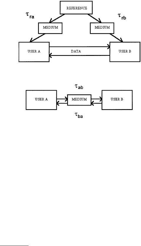
FIGURE 18.2 Common-view time transfer.
FIGURE 18.3 Two-way time transfer.
common to the reference cancel out, and the uncertainty caused by path delay is nearly eliminated. The result of the measurement is (Clock A – Clock B) – (τra – τrb).
Keep in mind that the common-view technique does not synchronize clocks in real time. The data must be exchanged with another user, and the results might not be known until long after the measurements are completed.
4.Two-way method: The two-way method requires two users to both transmit and receive through the same medium at the same time (Figure 18.3). Sites A and B simultaneously exchange time
signals through the same medium and compare the received signals with their own clocks. Site A
records A – (B + τba) and site B records B – (A + τab), where τba is the path delay from A to B, and τab is the path delay from A to B. The difference between these two sets of readings produces 2(A – B) – (τba – τab). If the path is reciprocal (τab = τba), then the difference, A – B, is known perfectly because the path between A and B has been measured. When properly implemented using a satellite
or fiber optic links, the two-way method outperforms all other time transfer methods and is capable of ±1 ns uncertainty.
Two-way time transfer has many potential applications in telecommunications networks. However, when a wireless medium is used, there are some restrictions that limit its usefulness. It might require expensive equipment and government licensing so that users can transmit. And like the common-view method, the two-way method requires users to exchange data. However, because users can transmit, it is possible to include the data with the timing information and to compute the results in real time.
5.Loop-back method: Like the two-way method, the loop-back method requires the receiver to send information back to the transmitter. For example, a time signal is sent from the transmitter (A)
©1999 by CRC Press LLC