Figure 9.36 Continued

and

Take, for example, an illustrative window as shown in Fig. 9.40. When i = 2,

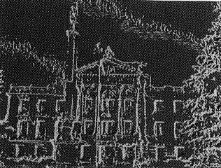
Figure 9.36 Continued

and

Similarly, we can get eight values for, i = 0, .... 7, as follows:

Figure 9.36 Continued

i	Si	Ti
0	7	13	4
1	3	17	36
2	3	17	36
3	3	17	36
4	7	13	4

(Continued)

Figure 9.37 Gradient image obtained by applying Sobel edge operator: (a) original image; (b) response of all horizontal edges; (c) response of all vertical edge elements; (d) response of all 45° edge elements; (e) response of all 135° edge elements; (f) response of all (s_z + s_y) edge elements; (g) response of (j« + s,_3S edge elements; (h) complete gradient image.

Figure 9.37 Continued

i	Si	Ti
5	11	9	28
6	15	5	60
7	11	9	28

Substitution of these values into Eq. (9.56) gives the gradient at the point G(j,k) = 60. It is not difficult to see from Eq. (8.56) that when the window is passed

Figure 9.37 Continued

into a smoothed region (i.e., with the same gray level in the neighbors as the center pixel), , i = 0, . . . , 7. Then the gradient G(j,k) at this center pixel will assume a value of 1. Basically, the Kirsch operator provides the maximal compass gradient magnitude about an image point [ignoring the pixel value of f(f,k)].

Wallis edge operator: This is a logarithmic Laplacian edge detector. The

Figure 9.37 Continued

principle of this detector is based on the homomorphic image processing. The assumption that Wallis made is that if the difference between the absolute value of the logarithm of the pixel luminance and the absolute value of the average of the logarithms of its four nearest neighbors is greater than a threshold value, an edge is assumed to exist.

Using the same window as that used by Kirsch (Fig. 9.40), an expression for G(j,k) can be put in the following form

Figure 9.38 Gradient image obtained by applying Sobel edge operator: (a) original image; (b) response of all horizontal edges; (c) response of all vertical edge elements; (d) response of all 45° edge elements; (e) response of all 135^o edge elements; (f) response of all (S_i + s_y) edge elements; (g) response of (s₄₅ + s₃₅) edge elements; (h) complete gradient image.

Figure 9.38 Continued

or

It can be seen that the logarithm does not have to be computed when compared

Figure 9.38 Continued

with the threshold. The computation will be simplified. In addition, this technique is insensitive to multiplicative change in the luminance level, since f(x,y)changes with ai, A₃, A_s, and A₇ by the same ratio.

Algorithm 6: least-square-fit operator. Before the image is processed, it is smoothed. Referring to Fig. 9.41, let f(x,y)) be the image model in the x у plane, and z = ax + by + c be a plane that fits the four points shown. The

Figure 9.38 Continued

Figure 9.39 Gradient image obtained by applying Sobel edge operator: (a) original image; (b) response of all horizontal edges; (c) response of all vertical edge elements; (d) response of all 45° edge elements; (e) response of all 135° edge elements; (f) response of all (s_x + s_y) edge elements; (g) response of (s₄₅ + s₁₃₅) edge elements; (h) complete gradient image.

Figure 9.39 Continued

error that resulted when z = ax + by + с is taken as the image plane will be the square root of Error², shown by the following equation:

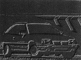
Figure 9.39 Continued

Figure 9.39 Continued

To optimize the solution, take ,and and set these partial derivatives to zero, a, b and с can then be found: