Image Enhancement (Spatial domain).

Image enhancement is an important step in the processing of large data sets to make the results more suitable for classification than were the original data. It accentuates and sharpens the image features, such as edges, boundaries, and contrast. The process docs not increase the inherent information content in the data, but it does increase the dynamic range of the features. Because of difficulties experienced in quantifying the criteria for enhancement, and the fact that image enhancement is so problem oriented, no general approaches arc available that can be used in every case, although lots of methods have been suggested.

The approaches suggested for enhancement can be grouped into two main categories: spatial processing and transform processing. In transform processing, the image function is first transformed to the transform domain and then processed to meet the specific problem requirements. Inverse transform is needed to yield the final spatial image results. On the other hand, with spatial domain processing, the pixels in the image are manipulated directly.

1. Deterministic Gray - Lever transformation

Processing in the spatial domain is usually carried out pixel by pixel. Depending on whether the processing is based only on the processed pixel or takes its neighboring pixels into consideration, processing can be further divided into two subcategories: point processing and neighborhood processing. With this defini­tion, the neighborhood used in point processing can be interpreted as being 1 X 1. In neighborhood processing, 3 x 3 or 5 x 5 windows are frequently used for the processing of a single pixel, and it is quite obvious that the com­putational time required will be greatly increased. Nevertheless,

f(x,y)

g(x,y)

g=T(f)

Conversion table or algebraic expression

such an increase in computational time is sometimes needed to obtain local context information, which is useful for decision making in specific pixel processing for certain purposes. For example, to smooth an image, we need to use the similarity property for a smooth region; to detect the boundary; we need to detect the sharp gray-level change between adjacent pixels.

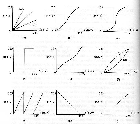
By point processing we mean that the processing of a certain pixel in the image depends on the information we have on that pixel itself, without consid­eration of the status of its neighborhood. There are several ways to treat this problem, one of which is deterministic gray-level transformation, and another, histogram modification. Deterministic gray-level transformation is quite straight­forward. A conversion table or algebraic expression will be stored, and the gray-level transformation for each pixel will be carried out either by table lookup or by algebraic computation, as shown schematically in Fig. 9.1, in which g(x,y) is (he image after gray-level transformation of the original image f(x,y). For an image of 512 x 512 pixels, 262,144 operations will be required. Figure 9.2 shows some of the deterministic gray-level transformations that could be used to meet various requirements. With the gray-level transformation function as shown in part (a), straight-line function 1 yields a brighter output than for the original, whereas straight-line function 2 gives a lower gray-level output for each pixel of the original image. Part (b) shows brightness stretching on the midregion of the image gray levels, part (c) gives a more eccentric action on this transformation which is useful in contrast stretching, and part (d) is the limiting transformation function, which yields a binary image (i.e., only two gray levels would exist in the image). Part (e) gives an effect opposite to that shown in part (b). In part (f), function 1 shows a dark region stretching trans­formation (i.e., dark becomes less dark, bright becomes less bright), and function 2 gives a bright region stretching transformation (i.e., lower gray-level outputs for lower gray levels of (f), but higher gray-level outputs for higher gray levels of (f). The sawtooth contrast scaling gray-level transformation function shown in part (g) can be used to produce a wide-dynamic-range image on a small-dynamic-range display. This is achieved by removing the most significant bit of the pixel value. Part (h) shows a reverse scaling, by means of which a negative of the original image can be obtained. Part (i) shows a thresholding transfor­mation,/where the height h can be changed to adjust the output dynamic range.