Figure 9.30 Robert’s cross-gradient operator.

gradient is large for prominent edges, small for a rather smooth area, and zero for a constant-gray-level area.

Several algorithms are available for performing edge sharpening:

Algorithm 1. Edge sharpening by selectively replacing a pixel point by its gradient. The algorithm can be put in the form shown in Fig. 9.31. The computation of can be done using the three-point gradient or the four-point gradient expression. When the value of is greater than or equal to a threshold, replace the pixel by its gradient value, or by gray level 255. Otherwise, keep it in the original level or a zero (or low) gray level. The process will run point by point through the 262,144 points from top to bottom and from left to right on the image.

Different gradient images can be generated from this algorithm depending on the values chosen for the g(j,k), j,k = 1,2, . . . ,N - 1, when its gradient >=Т and the values chosen for g(j,k) when < T. A binary gradient image will be obtained when the edges and background are displayed in 255 and 0. An edge-emphasized image without destroying the characteristics of smooth background can be obtained by

Algorithm 2. Edge sharpening by statistical differencing. The algorithm can be stated as follows:

(a) Specify a window (typically7x7 pixels) with the pixel (j,k) as the center.

(b) Compute the standard deviation  or variance ² over the elements inside the window.

where N is the number of pixels in the window and is the mean value of the original image in the window.

(c) Replace each pixel by a value g(j,k) which is the quotient of its original value divided by v(j,k) to generate the new image, such as

It can be noted that the enhanced image g(j,k) will be increased in amplitude with respect to the original image f(j,k) at the edge point and decreased elsewhere.

Algorithm 3. Edge sharpening by spatial convolution with a high-pass mask H such as

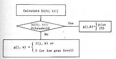
Figure 9.31 Algorithm for edge sharpening by selectively replacing pixel points by their gradients.

Examples of high-pass masks for edge sharpening are

The summation of the elements in each mask equals 1. The algorithm will be:

1. Examine all the pixels and compute g(j,k) by convolving f(j,k) with H.

2. Either use this computed value of g(j,k) as the new gray level of the pixel concerned or use the original value of f(j,k), depending on whether the difference between the computed g(j,k) and the original f(j,k) is greater than or less than the threshold chosen.

Other edge enhancement masks and operators have been suggested by various authors. These masks can be used to combine with the original image array to yield a two-dimensional discrete differentiation.

Compass gradient masks: These are so named because they indicate the slope directions of maximum responses, as shown by the dashed angle in Fig. 9.3