vk.com/club152685050Modeling Species Transport| vkand.com/id446425943Gaseous Combustion

d. Close the Surface Integrals dialog box.

13.5.9. NOx Prediction

In this section you will extend the ANSYS Fluent model to include the prediction of NOx. You will first calculate the formation of both thermal and prompt NOx, then calculate each separately to determine the contribution of each mechanism.

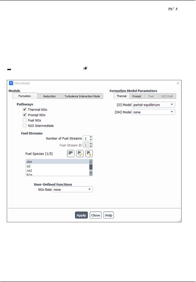
1. Enable the NOx model.

Setup → Models → Species → NOx Edit...

a.Enable Thermal NOx and Prompt NOx in the Pathways group box.

b.Select ch4 from the Fuel Species selection list.

c.Click the Turbulence Interaction Mode tab.

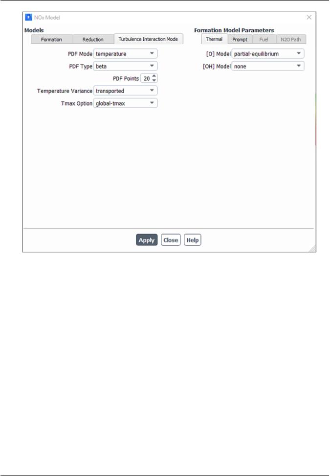
i.Select temperature from the PDF Mode drop-down list.

This will enable the turbulence-chemistry interaction. If turbulence interaction is not enabled, you will be computing NOx formation without considering the important influence of turbulent fluctuations on the time-averaged reaction rates.

ii.Retain the default selection of beta from the PDF Type drop-down list and enter 20 for PDF Points.

The value for PDF Points is increased from 10 to 20 to obtain a more accurate NOx prediction.

iii.Select transported from the Temperature Variance drop-down list.

d.Select partial-equilibrium from the [O] Model drop-down list in the Formation Model Parameters group box in the Thermal tab.

The partial-equilibrium model is used to predict the O radical concentration required for thermal NOx prediction.

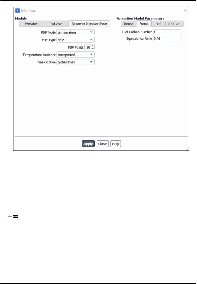
e.Click the Prompt tab.

vk.com/club152685050Modeling Species Transport| vkand.com/id446425943Gaseous Combustion

i.Retain the default value of 1 for Fuel Carbon Number.

ii.Enter 0.76 for Equivalence Ratio.

All of the parameters in the Prompt tab are used in the calculation of prompt NOx formation. The Fuel Carbon Number is the number of carbon atoms per molecule of fuel. The Equivalence Ratio defines the fuel-air ratio (relative to stoichiometric conditions).

f.Click Apply to accept these changes and close the NOx Model dialog box.

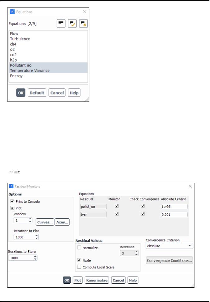
2.Enable the calculation of NO species only and temperature variance.

Solution → Controls → Equations...

a.Deselect all variables except Pollutant no and Temperature Variance from the Equations selection list.

b.Click OK to close the Equations dialog box.

You will predict NOx formation in a “postprocessing” mode, with the flow field, temperature, and hydrocarbon combustion species concentrations fixed. Hence, only the NO equation will be computed. Prediction of NO in this mode is justified on the grounds that the NO concentrations are very low and have negligible impact on the hydrocarbon combustion prediction.

3.Confirm the convergence criterion for the NO species equation.

Solution → Reports → Residuals...

vk.com/club152685050Modeling Species Transport| vkand.com/id446425943Gaseous Combustion

a.Ensure that the Absolute Criteria for pollut_no is set to 1e-06.

b.Click OK to close the Residual Monitors dialog box.

4.Request 25 more iterations.

Solution → Run Calculation

5.Save the new case and data files (gascomb2.cas.gz and gascomb2.dat.gz).

File → Write → Case & Data...

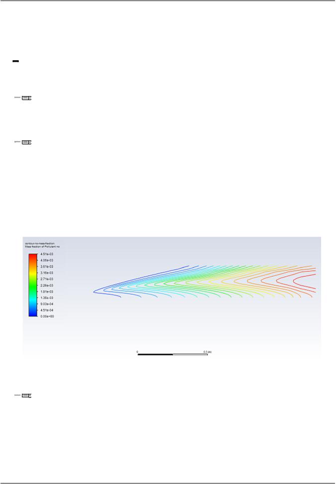
6.Review the solution by creating and displaying a contour definition for NO mass fraction (Figure 13.9: Contours of NO Mass Fraction — Prompt and Thermal NOx Formation (p. 474)).

Results → Graphics → Contours → New...

a.Enter contour-no-mass-fraction for Contour Name.

b.Disable Filled in the Options group box.

c.Select NOx... and Mass fraction of Pollutant no from the Contours of drop-down lists.

d.Click Save/Display and close the Contours dialog box.

Figure 13.9: Contours of NO Mass Fraction — Prompt and Thermal NOx Formation

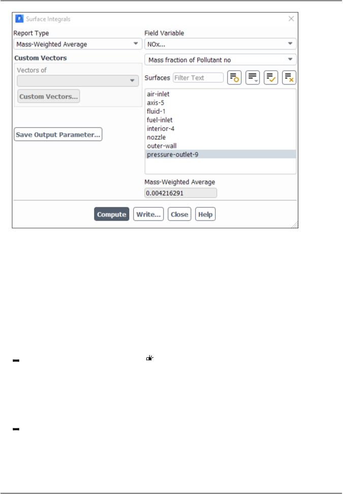
7.Calculate the average exit NO mass fraction.

Results → Reports → Surface Integrals...

a.Select Mass-Weighted Average from the Report Type drop-down list.

b.Select NOx... and Mass fraction of Pollutant no from the Field Variable drop-down lists.

c.Ensure that pressure-outlet-9 is selected from the Surfaces selection list.

d.Click Compute.

The Mass-Weighted Average field will show that the exit NO mass fraction is approximately 0.00421.

e.Close the Surface Integrals dialog box.

8.Disable the prompt NOx mechanism in preparation for solving for thermal NOx only.

Setup → Models → Species → NOx Edit...

a.In the Formation tab, disable Prompt NOx.

b.Click Apply and close the NOx Model dialog box.

9.Request 25 iterations.

Solution → Run Calculation

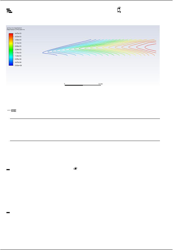
10.Review the thermal NOx solution by displaying the contour-no-mass-fraction contour definition for NO mass fraction (under the Results/Graphics/Contours tree branch) you created earlier (Figure 13.10: Contours of NO Mass Fraction—Thermal NOx Formation (p. 476)).

vk.com/club152685050Modeling Species Transport| vkand.com/id446425943Gaseous Combustion

Figure 13.10: Contours of NO Mass Fraction—Thermal NOx Formation

Note that the concentration of NO is slightly lower without the prompt NOx mechanism.

11.Compute the average exit NO mass fraction with only thermal NOx formation.

Results → Reports → Surface Integrals...

Tip

Follow the same procedure you used earlier for the calculation with both thermal and prompt NOx formation.

The Mass-Weighted Average field will show that the exit NO mass fraction with only thermal NOx formation (without prompt NOx formation) is approximately 0.004176.

12. Solve for prompt NOx production only.

Setup → Models → Species → NOx Edit...

a.Disable Thermal NOx in the Pathways group box.

b.Enable Prompt NOx.

c.Click Apply and close the NOx Model dialog box.

13.Request 25 iterations.

Solution → Run Calculation

14.Review the prompt NOx solution by displaying the contour-no-mass-fraction contour definition for NO mass fraction (under the Results/Graphics/Contours tree branch) (Figure 13.11: Contours of NO Mass Fraction—Prompt NOx Formation (p. 477)).

Figure 13.11: Contours of NO Mass Fraction—Prompt NOx Formation

The prompt NOx mechanism is most significant in fuel-rich flames. In this case the flame is lean and prompt NO production is low.

15.Compute the average exit NO mass fraction only with prompt NOx formation.

Results → Reports → Surface Integrals...

Tip

Follow the same procedure you used earlier for the calculation with both thermal and prompt NOx formation.

The Mass-Weighted Average field will show that the exit NO mass fraction with only prompt NOx formation is approximately 9.9775e-05.

Note

The individual thermal and prompt NO mass fractions do not add up to the levels predicted with the two models combined. This is because reversible reactions are involved. NO produced in one reaction can be destroyed in another reaction.

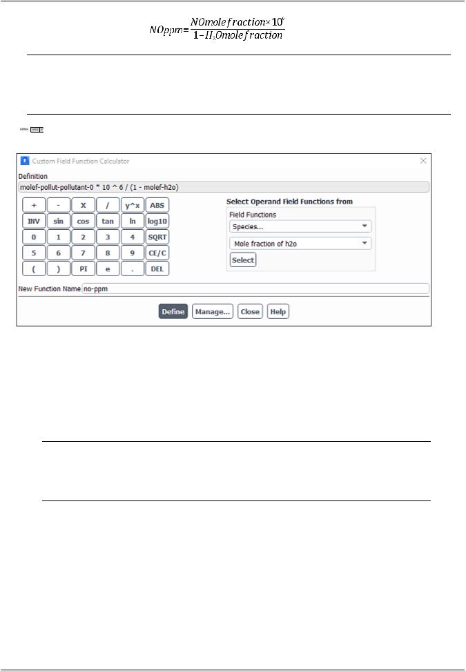
16.Use a custom field function to compute NO parts per million (ppm).

The NOppm will be computed from the following equation:

vk.com/club152685050Modeling Species Transport| vkand.com/id446425943Gaseous Combustion

(13.4)

Note

This is the dry ppm. Therefore, the value is normalized by removing the water mole fraction in the denominator.

User Defined → Field Functions → Custom...

a.Select NOx... and Mole fraction of Pollutant no from the Field Functions drop-down lists, and click the Select button to enter molef-pollut-pollutant-0 in the Definition field.

b.Click the appropriate calculator buttons to enter

*10ˆ6/(1-

in the Definition field, as shown in the previous dialog box.

Tip

If you make a mistake, click the DEL button on the calculator pad to delete the last item you added to the function definition.

For more explicit instructions on using the Custom Field Function calculator buttons, see Fluid Flow and Heat Transfer in a Mixing Elbow (p. 35).

c.Select Species... and Mole fraction of h2o from the Field Functions drop-down lists, and click the

Select button to enter molef-h2o in the Definition field.

d.Click the ) button to complete the field function.

e.Enter no-ppm for New Function Name.

f.Click Define to add the new field function to the variable list and close the Custom Field Function Calculator dialog box.