Figure 3.5: Display with Additional Lighting

h. Close the Lights dialog box.

Extra

You can use the left mouse button to rotate the ball in the Active Lights window to gain a perspective view on the relative locations of the lights that are currently active, and see the shading effect on the ball at the center.

You can also change the color of one or more of the lights by selecting the color from the Color drop-down list or by moving the Red, Green, and Blue sliders.

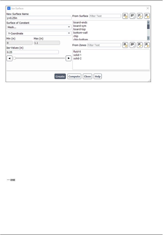
3.4.5. Creating Isosurfaces

To display results in a 3D model, you will need surfaces on which the data can be displayed. Fluent creates surfaces for all boundary zones automatically. Several surfaces have been renamed after reading the case file. Examples are board-sym and board-ends, which correspond to the side and end faces of the circuit board.

You can define additional surfaces for viewing the results, such as a plane in Cartesian space. In this exercise, you will create a horizontal plane cutting through the middle of the module with a Y value of 0.25 inches. You can use this surface to display the temperature and velocity fields.

1.Create a surface of constant Y coordinate.

Results → Surface → Create → Iso-Surface...

vk.com/club152685050Postprocessing | vk.com/id446425943

a. Enter y=0.25in for New Surface Name.

Tip

When you are creating multiple postprocessing surfaces, it can be helpful to group

surfaces by type for viewing in lists (Click and select Surface Type under Group By). All iso-surfaces will be grouped together.

b.Select Mesh... and Y-Coordinate from the Surface of Constant drop-down lists.

c.Click Compute.

The Min and Max fields display the Y extents of the domain.

d.Enter 0.25 for Iso-Values.

e.Click Create and close the Iso-Surface dialog box.

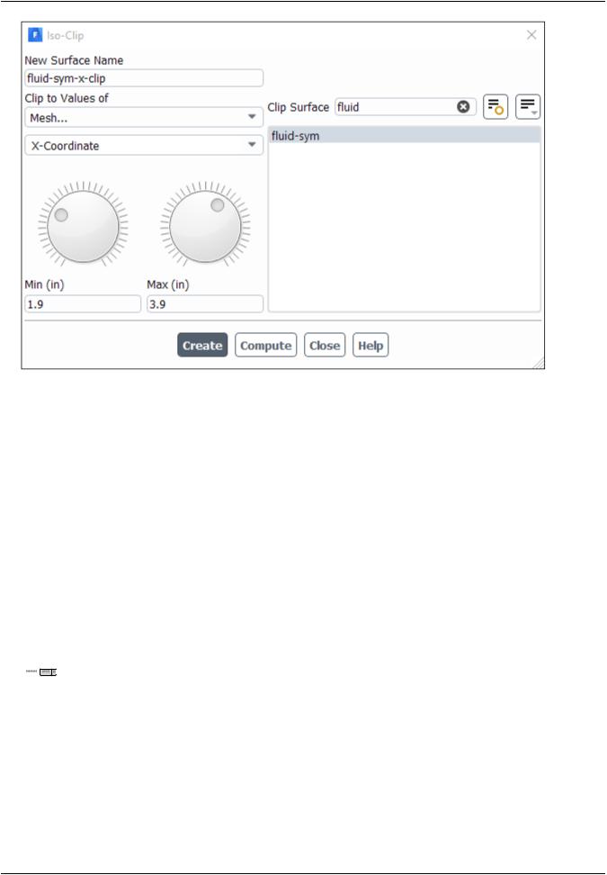
2.Create a clipped surface for the X coordinate of the fluid (fluid-sym).

Domain → Surface → Create → Iso-Clip...

a.Enter fluid-sym-x-clip for New Surface Name.

b.Select Mesh... and X-Coordinate from the Clip to Values of drop-down lists.

c.Select fluid-sym from the Clip Surface selection list. You can type fluid into the Filter Text box to quickly find this surface.

d.Click Compute.

The Min and Max fields display the X extents of the domain.

e.Enter 1.9 and 3.9 for Min and Max respectively.

This will isolate the area around the chip.

f.Click Create.

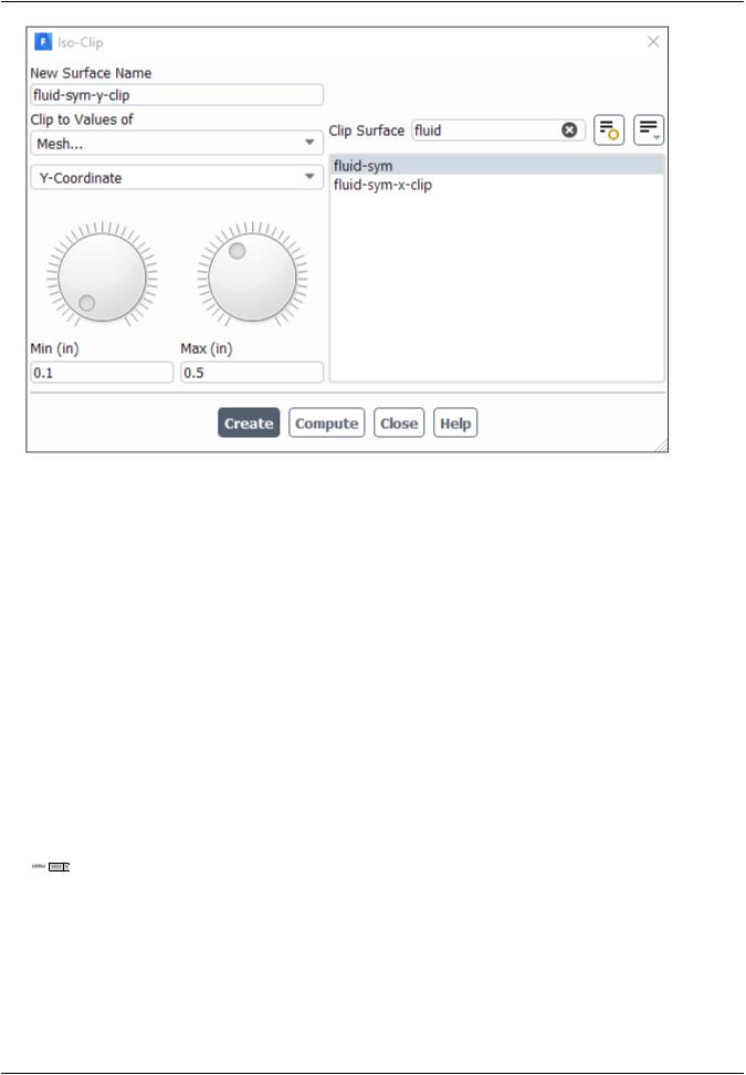
3.Create a clipped surface for the Y coordinate of the fluid (fluid-sym).

Domain → Surface → Create → Iso-Clip...

vk.com/club152685050Postprocessing | vk.com/id446425943

a.Enter fluid-sym-y-clip for New Surface Name.

b.Select Mesh... and Y-Coordinate from the Clip to Values of drop-down lists.

c.Retain the selection of fluid-sym from the Clip Surface selection list.

d.Click Compute.

The Min and Max fields display the Y extents of the domain.

e.Enter 0.1 and 0.5 for Min and Max respectively.

This will isolate the area around the chip.

f.Click Create and close the Iso-Clip dialog box.

3.4.6.Generating Contours

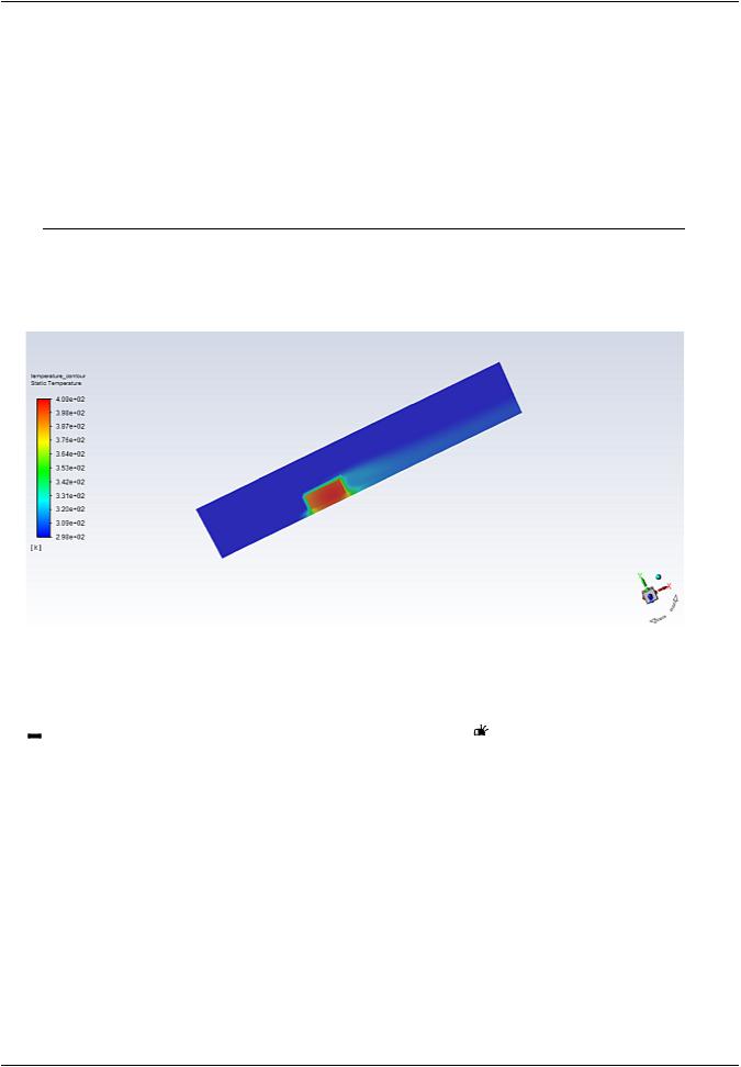
1.Display filled contours of temperature on the symmetry plane (Figure 3.6: Filled Contours of Temperature on the Symmetry Surfaces (p. 108)).

Results → Graphics → Contours → New...

a.Enter temperature_contour for Contour Name.

b.Ensure Filled, Node Values, Global Range, and Auto Range are enabled in the Options group box.

c.Select Smooth for Coloring.

d.Select Temperature... and Static Temperature from the Contours of drop-down lists.

e.Click and select Surface Type under Group By (if surfaces are not already grouped by type).

f.Select board-sym, chip-sym, and fluid-sym (under Symmetry in the Surfaces selection list.)

g.Click Save/Display.

h.Rotate and adjust the magnification of the view using the left and middle mouse buttons, respectively, to obtain the view as shown in Figure 3.6: Filled Contours of Temperature on the Symmetry Sur-

faces (p. 108).

Tip

If the model disappears from the graphics window at any time, or if you are having difficulty manipulating it with the mouse, do one of the following:

vk.com/club152685050Postprocessing | vk.com/id446425943

•Click the Fit to Window button in the graphics toolbar.

•Open the Views dialog box by right-clicking Graphics in the tree (under Results) and selecting Views... from the menu that opens, and then use the Default button to reset the view. You could also click Camera... in this dialog box to open the Camera Parameters dialog box, where you could select orthographic from the Projection drop-down list to reduce the likelihood of zooming through the geometry.

•Press the Ctrl + L to revert to a previous view.

The peak temperatures in the chip appear where the heat is generated, along with the higher temperatures in the wake where the flow is recirculating.

Figure 3.6: Filled Contours of Temperature on the Symmetry Surfaces

2.Display filled contours of temperature for the clipped surface (Figure 3.7: Filled Contours of Temperature on the Clipped Surface (p. 109)).

Results → Graphics → Contours → temperature_contour Edit...

a.Click to deselect all surfaces from the Surfaces selection list and then select fluid-sym-x-clip and fluid-sym-y-clip.

b.Click Save/Display.

A clipped surface appears, colored by temperature (Figure 3.7: Filled Contours of Temperature on the Clipped Surface (p. 109)).

Figure 3.7: Filled Contours of Temperature on the Clipped Surface

3. Display filled contours of temperature on the plane, y=0.25in (Figure 3.8: Temperature Contours on the Surface, Y= 0.25 in. (p. 110)).

a.Click to deselect all surfaces from the Surfaces selection list and then select y=0.25in.

b.Click Save/Display and close the Contours dialog box.

The filled temperature contours will be displayed on the y=0.25in plane.

c.Orient the view to display the contours.

4.Change the location of the colormap in the graphics window.

Left-click the colormap in the graphics window and drag it to the bottom of the graphics window.

This can also be accomplished using the Display Options dialog box.

Tip

You can increase/decrease the size of the colormap by dragging the corners of the box that appears when you hover over the colormap.