

- •ANSYS Fluent Tutorial Guide
- •Table of Contents
- •Using This Manual
- •1. What’s In This Manual
- •2. How To Use This Manual
- •2.1. For the Beginner
- •2.2. For the Experienced User
- •3. Typographical Conventions Used In This Manual
- •Chapter 1: Fluid Flow in an Exhaust Manifold
- •1.1. Introduction
- •1.2. Prerequisites
- •1.3. Problem Description
- •1.4. Setup and Solution
- •1.4.1. Preparation
- •1.4.2. Meshing Workflow
- •1.4.3. General Settings
- •1.4.4. Solver Settings
- •1.4.5. Models
- •1.4.6. Materials
- •1.4.7. Cell Zone Conditions
- •1.4.8. Boundary Conditions
- •1.4.9. Solution
- •1.4.10. Postprocessing
- •1.5. Summary
- •Chapter 2: Fluid Flow and Heat Transfer in a Mixing Elbow
- •2.1. Introduction
- •2.2. Prerequisites
- •2.3. Problem Description
- •2.4. Setup and Solution
- •2.4.1. Preparation
- •2.4.2. Launching ANSYS Fluent
- •2.4.3. Reading the Mesh
- •2.4.4. Setting Up Domain
- •2.4.5. Setting Up Physics
- •2.4.6. Solving
- •2.4.7. Displaying the Preliminary Solution
- •2.4.8. Adapting the Mesh
- •2.5. Summary
- •Chapter 3: Postprocessing
- •3.1. Introduction
- •3.2. Prerequisites
- •3.3. Problem Description
- •3.4. Setup and Solution
- •3.4.1. Preparation
- •3.4.2. Reading the Mesh
- •3.4.3. Manipulating the Mesh in the Viewer
- •3.4.4. Adding Lights
- •3.4.5. Creating Isosurfaces
- •3.4.6. Generating Contours
- •3.4.7. Generating Velocity Vectors
- •3.4.8. Creating an Animation
- •3.4.9. Displaying Pathlines
- •3.4.10. Creating a Scene With Vectors and Contours
- •3.4.11. Advanced Overlay of Pathlines on a Scene
- •3.4.12. Creating Exploded Views
- •3.4.13. Animating the Display of Results in Successive Streamwise Planes
- •3.4.14. Generating XY Plots
- •3.4.15. Creating Annotation
- •3.4.16. Saving Picture Files
- •3.4.17. Generating Volume Integral Reports
- •3.5. Summary
- •Chapter 4: Modeling Periodic Flow and Heat Transfer
- •4.1. Introduction
- •4.2. Prerequisites
- •4.3. Problem Description
- •4.4. Setup and Solution
- •4.4.1. Preparation
- •4.4.2. Mesh
- •4.4.3. General Settings
- •4.4.4. Models
- •4.4.5. Materials
- •4.4.6. Cell Zone Conditions
- •4.4.7. Periodic Conditions
- •4.4.8. Boundary Conditions
- •4.4.9. Solution
- •4.4.10. Postprocessing
- •4.5. Summary
- •4.6. Further Improvements
- •Chapter 5: Modeling External Compressible Flow
- •5.1. Introduction
- •5.2. Prerequisites
- •5.3. Problem Description
- •5.4. Setup and Solution
- •5.4.1. Preparation
- •5.4.2. Mesh
- •5.4.3. Solver
- •5.4.4. Models
- •5.4.5. Materials
- •5.4.6. Boundary Conditions
- •5.4.7. Operating Conditions
- •5.4.8. Solution
- •5.4.9. Postprocessing
- •5.5. Summary
- •5.6. Further Improvements
- •Chapter 6: Modeling Transient Compressible Flow
- •6.1. Introduction
- •6.2. Prerequisites
- •6.3. Problem Description
- •6.4. Setup and Solution
- •6.4.1. Preparation
- •6.4.2. Reading and Checking the Mesh
- •6.4.3. Solver and Analysis Type
- •6.4.4. Models
- •6.4.5. Materials
- •6.4.6. Operating Conditions
- •6.4.7. Boundary Conditions
- •6.4.8. Solution: Steady Flow
- •6.4.9. Enabling Time Dependence and Setting Transient Conditions
- •6.4.10. Specifying Solution Parameters for Transient Flow and Solving
- •6.4.11. Saving and Postprocessing Time-Dependent Data Sets
- •6.5. Summary
- •6.6. Further Improvements
- •Chapter 7: Modeling Flow Through Porous Media
- •7.1. Introduction
- •7.2. Prerequisites
- •7.3. Problem Description
- •7.4. Setup and Solution
- •7.4.1. Preparation
- •7.4.2. Mesh
- •7.4.3. General Settings
- •7.4.4. Models
- •7.4.5. Materials
- •7.4.6. Cell Zone Conditions
- •7.4.7. Boundary Conditions
- •7.4.8. Solution
- •7.4.9. Postprocessing
- •7.5. Summary
- •7.6. Further Improvements
- •Chapter 8: Modeling Radiation and Natural Convection
- •8.1. Introduction
- •8.2. Prerequisites
- •8.3. Problem Description
- •8.4. Setup and Solution
- •8.4.1. Preparation
- •8.4.2. Reading and Checking the Mesh
- •8.4.3. Solver and Analysis Type
- •8.4.4. Models
- •8.4.5. Defining the Materials
- •8.4.6. Operating Conditions
- •8.4.7. Boundary Conditions
- •8.4.8. Obtaining the Solution
- •8.4.9. Postprocessing
- •8.4.10. Comparing the Contour Plots after Varying Radiating Surfaces
- •8.4.11. S2S Definition, Solution, and Postprocessing with Partial Enclosure
- •8.5. Summary
- •8.6. Further Improvements
- •Chapter 9: Using a Single Rotating Reference Frame
- •9.1. Introduction
- •9.2. Prerequisites
- •9.3. Problem Description
- •9.4. Setup and Solution
- •9.4.1. Preparation
- •9.4.2. Mesh
- •9.4.3. General Settings
- •9.4.4. Models
- •9.4.5. Materials
- •9.4.6. Cell Zone Conditions
- •9.4.7. Boundary Conditions
- •9.4.8. Solution Using the Standard k- ε Model
- •9.4.9. Postprocessing for the Standard k- ε Solution
- •9.4.10. Solution Using the RNG k- ε Model
- •9.4.11. Postprocessing for the RNG k- ε Solution
- •9.5. Summary
- •9.6. Further Improvements
- •9.7. References
- •Chapter 10: Using Multiple Reference Frames
- •10.1. Introduction
- •10.2. Prerequisites
- •10.3. Problem Description
- •10.4. Setup and Solution
- •10.4.1. Preparation
- •10.4.2. Mesh
- •10.4.3. Models
- •10.4.4. Materials
- •10.4.5. Cell Zone Conditions
- •10.4.6. Boundary Conditions
- •10.4.7. Solution
- •10.4.8. Postprocessing
- •10.5. Summary
- •10.6. Further Improvements
- •Chapter 11: Using Sliding Meshes
- •11.1. Introduction
- •11.2. Prerequisites
- •11.3. Problem Description
- •11.4. Setup and Solution
- •11.4.1. Preparation
- •11.4.2. Mesh
- •11.4.3. General Settings
- •11.4.4. Models
- •11.4.5. Materials
- •11.4.6. Cell Zone Conditions
- •11.4.7. Boundary Conditions
- •11.4.8. Operating Conditions
- •11.4.9. Mesh Interfaces
- •11.4.10. Solution
- •11.4.11. Postprocessing
- •11.5. Summary
- •11.6. Further Improvements
- •Chapter 12: Using Overset and Dynamic Meshes
- •12.1. Prerequisites
- •12.2. Problem Description
- •12.3. Preparation
- •12.4. Mesh
- •12.5. Overset Interface Creation
- •12.6. Steady-State Case Setup
- •12.6.1. General Settings
- •12.6.2. Models
- •12.6.3. Materials
- •12.6.4. Operating Conditions
- •12.6.5. Boundary Conditions
- •12.6.6. Reference Values
- •12.6.7. Solution
- •12.7. Unsteady Setup
- •12.7.1. General Settings
- •12.7.2. Compile the UDF
- •12.7.3. Dynamic Mesh Settings
- •12.7.4. Report Generation for Unsteady Case
- •12.7.5. Run Calculations for Unsteady Case
- •12.7.6. Overset Solution Checking
- •12.7.7. Postprocessing
- •12.7.8. Diagnosing an Overset Case
- •12.8. Summary
- •Chapter 13: Modeling Species Transport and Gaseous Combustion
- •13.1. Introduction
- •13.2. Prerequisites
- •13.3. Problem Description
- •13.4. Background
- •13.5. Setup and Solution
- •13.5.1. Preparation
- •13.5.2. Mesh
- •13.5.3. General Settings
- •13.5.4. Models
- •13.5.5. Materials
- •13.5.6. Boundary Conditions
- •13.5.7. Initial Reaction Solution
- •13.5.8. Postprocessing
- •13.5.9. NOx Prediction
- •13.6. Summary
- •13.7. Further Improvements
- •Chapter 14: Using the Eddy Dissipation and Steady Diffusion Flamelet Combustion Models
- •14.1. Introduction
- •14.2. Prerequisites
- •14.3. Problem Description
- •14.4. Setup and Solution
- •14.4.1. Preparation
- •14.4.2. Mesh
- •14.4.3. Solver Settings
- •14.4.4. Models
- •14.4.5. Boundary Conditions
- •14.4.6. Solution
- •14.4.7. Postprocessing for the Eddy-Dissipation Solution
- •14.5. Steady Diffusion Flamelet Model Setup and Solution
- •14.5.1. Models
- •14.5.2. Boundary Conditions
- •14.5.3. Solution
- •14.5.4. Postprocessing for the Steady Diffusion Flamelet Solution
- •14.6. Summary
- •Chapter 15: Modeling Surface Chemistry
- •15.1. Introduction
- •15.2. Prerequisites
- •15.3. Problem Description
- •15.4. Setup and Solution
- •15.4.1. Preparation
- •15.4.2. Reading and Checking the Mesh
- •15.4.3. Solver and Analysis Type
- •15.4.4. Specifying the Models
- •15.4.5. Defining Materials and Properties
- •15.4.6. Specifying Boundary Conditions
- •15.4.7. Setting the Operating Conditions
- •15.4.8. Simulating Non-Reacting Flow
- •15.4.9. Simulating Reacting Flow
- •15.4.10. Postprocessing the Solution Results
- •15.5. Summary
- •15.6. Further Improvements
- •Chapter 16: Modeling Evaporating Liquid Spray
- •16.1. Introduction
- •16.2. Prerequisites
- •16.3. Problem Description
- •16.4. Setup and Solution
- •16.4.1. Preparation
- •16.4.2. Mesh
- •16.4.3. Solver
- •16.4.4. Models
- •16.4.5. Materials
- •16.4.6. Boundary Conditions
- •16.4.7. Initial Solution Without Droplets
- •16.4.8. Creating a Spray Injection
- •16.4.9. Solution
- •16.4.10. Postprocessing
- •16.5. Summary
- •16.6. Further Improvements
- •Chapter 17: Using the VOF Model
- •17.1. Introduction
- •17.2. Prerequisites
- •17.3. Problem Description
- •17.4. Setup and Solution
- •17.4.1. Preparation
- •17.4.2. Reading and Manipulating the Mesh
- •17.4.3. General Settings
- •17.4.4. Models
- •17.4.5. Materials
- •17.4.6. Phases
- •17.4.7. Operating Conditions
- •17.4.8. User-Defined Function (UDF)
- •17.4.9. Boundary Conditions
- •17.4.10. Solution
- •17.4.11. Postprocessing
- •17.5. Summary
- •17.6. Further Improvements
- •Chapter 18: Modeling Cavitation
- •18.1. Introduction
- •18.2. Prerequisites
- •18.3. Problem Description
- •18.4. Setup and Solution
- •18.4.1. Preparation
- •18.4.2. Reading and Checking the Mesh
- •18.4.3. Solver Settings
- •18.4.4. Models
- •18.4.5. Materials
- •18.4.6. Phases
- •18.4.7. Boundary Conditions
- •18.4.8. Operating Conditions
- •18.4.9. Solution
- •18.4.10. Postprocessing
- •18.5. Summary
- •18.6. Further Improvements
- •Chapter 19: Using the Multiphase Models
- •19.1. Introduction
- •19.2. Prerequisites
- •19.3. Problem Description
- •19.4. Setup and Solution
- •19.4.1. Preparation
- •19.4.2. Mesh
- •19.4.3. Solver Settings
- •19.4.4. Models
- •19.4.5. Materials
- •19.4.6. Phases
- •19.4.7. Cell Zone Conditions
- •19.4.8. Boundary Conditions
- •19.4.9. Solution
- •19.4.10. Postprocessing
- •19.5. Summary
- •Chapter 20: Modeling Solidification
- •20.1. Introduction
- •20.2. Prerequisites
- •20.3. Problem Description
- •20.4. Setup and Solution
- •20.4.1. Preparation
- •20.4.2. Reading and Checking the Mesh
- •20.4.3. Specifying Solver and Analysis Type
- •20.4.4. Specifying the Models
- •20.4.5. Defining Materials
- •20.4.6. Setting the Cell Zone Conditions
- •20.4.7. Setting the Boundary Conditions
- •20.4.8. Solution: Steady Conduction
- •20.5. Summary
- •20.6. Further Improvements
- •Chapter 21: Using the Eulerian Granular Multiphase Model with Heat Transfer
- •21.1. Introduction
- •21.2. Prerequisites
- •21.3. Problem Description
- •21.4. Setup and Solution
- •21.4.1. Preparation
- •21.4.2. Mesh
- •21.4.3. Solver Settings
- •21.4.4. Models
- •21.4.6. Materials
- •21.4.7. Phases
- •21.4.8. Boundary Conditions
- •21.4.9. Solution
- •21.4.10. Postprocessing
- •21.5. Summary
- •21.6. Further Improvements
- •21.7. References
- •22.1. Introduction
- •22.2. Prerequisites
- •22.3. Problem Description
- •22.4. Setup and Solution
- •22.4.1. Preparation
- •22.4.2. Structural Model
- •22.4.3. Materials
- •22.4.4. Cell Zone Conditions
- •22.4.5. Boundary Conditions
- •22.4.6. Solution
- •22.4.7. Postprocessing
- •22.5. Summary
- •23.1. Introduction
- •23.2. Prerequisites
- •23.3. Problem Description
- •23.4. Setup and Solution
- •23.4.1. Preparation
- •23.4.2. Solver and Analysis Type
- •23.4.3. Structural Model
- •23.4.4. Materials
- •23.4.5. Cell Zone Conditions
- •23.4.6. Boundary Conditions
- •23.4.7. Dynamic Mesh Zones
- •23.4.8. Solution Animations
- •23.4.9. Solution
- •23.4.10. Postprocessing
- •23.5. Summary
- •Chapter 24: Using the Adjoint Solver – 2D Laminar Flow Past a Cylinder
- •24.1. Introduction
- •24.2. Prerequisites
- •24.3. Problem Description
- •24.4. Setup and Solution
- •24.4.1. Step 1: Preparation
- •24.4.2. Step 2: Define Observables
- •24.4.3. Step 3: Compute the Drag Sensitivity
- •24.4.4. Step 4: Postprocess and Export Drag Sensitivity
- •24.4.4.1. Boundary Condition Sensitivity
- •24.4.4.2. Momentum Source Sensitivity
- •24.4.4.3. Shape Sensitivity
- •24.4.4.4. Exporting Drag Sensitivity Data
- •24.4.5. Step 5: Compute Lift Sensitivity
- •24.4.6. Step 6: Modify the Shape
- •24.5. Summary
- •25.1. Introduction
- •25.2. Prerequisites
- •25.3. Problem Description
- •25.4. Setup and Solution
- •25.4.1. Preparation
- •25.4.2. Reading and Scaling the Mesh
- •25.4.3. Loading the MSMD battery Add-on
- •25.4.4. NTGK Battery Model Setup
- •25.4.4.1. Specifying Solver and Models
- •25.4.4.2. Defining New Materials for Cell and Tabs
- •25.4.4.3. Defining Cell Zone Conditions
- •25.4.4.4. Defining Boundary Conditions
- •25.4.4.5. Specifying Solution Settings
- •25.4.4.6. Obtaining Solution
- •25.4.5. Postprocessing
- •25.4.6. Simulating the Battery Pulse Discharge Using the ECM Model
- •25.4.7. Using the Reduced Order Method (ROM)
- •25.4.8. External and Internal Short-Circuit Treatment
- •25.4.8.1. Setting up and Solving a Short-Circuit Problem
- •25.4.8.2. Postprocessing
- •25.5. Summary
- •25.6. Appendix
- •25.7. References
- •26.1. Introduction
- •26.2. Prerequisites
- •26.3. Problem Description
- •26.4. Setup and Solution
- •26.4.1. Preparation
- •26.4.2. Reading and Scaling the Mesh
- •26.4.3. Loading the MSMD battery Add-on
- •26.4.4. Battery Model Setup
- •26.4.4.1. Specifying Solver and Models
- •26.4.4.2. Defining New Materials
- •26.4.4.3. Defining Cell Zone Conditions
- •26.4.4.4. Defining Boundary Conditions
- •26.4.4.5. Specifying Solution Settings
- •26.4.4.6. Obtaining Solution
- •26.4.5. Postprocessing
- •26.5. Summary
- •Chapter 27: In-Flight Icing Tutorial Using Fluent Icing
- •27.1. Fluent Airflow on the NACA0012 Airfoil
- •27.2. Flow Solution on the Rough NACA0012 Airfoil
- •27.3. Droplet Impingement on the NACA0012
- •27.3.1. Monodispersed Calculation
- •27.3.2. Langmuir-D Distribution
- •27.3.3. Post-Processing Using Quick-View
- •27.4. Fluent Icing Ice Accretion on the NACA0012
- •27.5. Postprocessing an Ice Accretion Solution Using CFD-Post Macros
- •27.6. Multi-Shot Ice Accretion with Automatic Mesh Displacement
- •27.7. Multi-Shot Ice Accretion with Automatic Mesh Displacement – Postprocessing Using CFD-Post
vk.com/club152685050Using Sliding Meshes | vk.com/id446425943
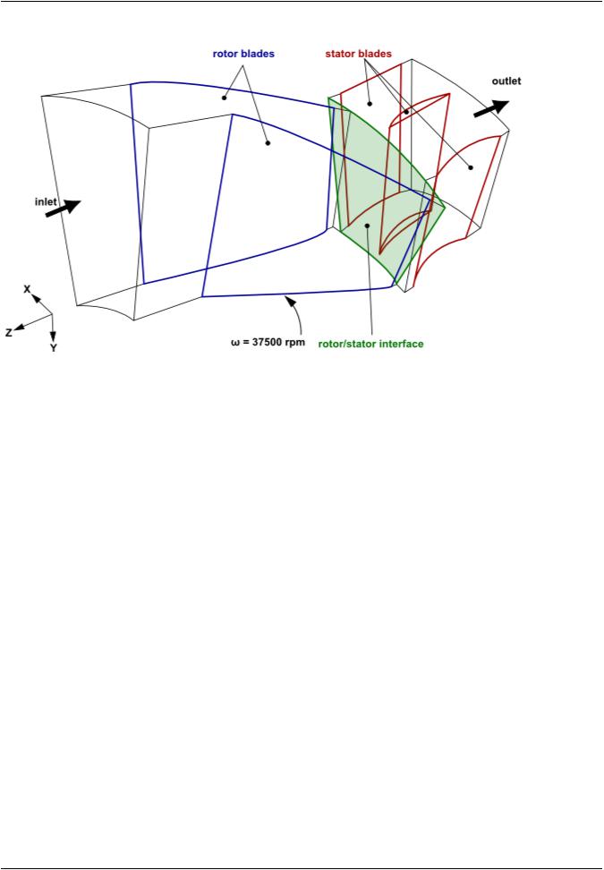
Figure 11.1: Rotor-Stator Problem Description
11.4. Setup and Solution
The following sections describe the setup and solution steps for this tutorial:
11.4.1.Preparation
11.4.2.Mesh
11.4.3.General Settings
11.4.4.Models
11.4.5.Materials
11.4.6.Cell Zone Conditions
11.4.7.Boundary Conditions
11.4.8.Operating Conditions
11.4.9.Mesh Interfaces
11.4.10.Solution
11.4.11.Postprocessing
11.4.1. Preparation
To prepare for running this tutorial:
1.Download the sliding_mesh.zip file here.
2.Unzip sliding_mesh.zip to your working directory.
3.The mesh file axial_comp.msh can be found in the folder.
4.Use Fluent Launcher to start the 3D version of ANSYS Fluent.
Fluent Launcher displays your Display Options preferences from the previous session.
For more information about Fluent Launcher, see starting ANSYS Fluent using the Fluent Launcher in the Fluent Getting Started Guide.
|
Release 2019 R1 - © ANSYS,Inc.All rights reserved.- Contains proprietary and confidential information |
368 |
of ANSYS, Inc. and its subsidiaries and affiliates. |

vk.com/club152685050 | vk.com/id446425943 |
Setup and Solution |
5.Ensure that the Display Mesh After Reading option is enabled.
6.Enable single precision (disable Double Precision).
7.Do not enable Meshing Mode.
8.Run in Serial under Processing Options.
11.4.2. Mesh
1. Read in the mesh file axial_comp.msh.

 File → Read → Mesh...
11.4.3. General Settings
1.Check the mesh.
 Domain → Mesh → Check → Perform Mesh Check
ANSYS Fluent will perform various checks on the mesh and will report the progress in the console. Ensure that the reported minimum volume is a positive number.
Warnings will be displayed regarding unassigned interface zones, resulting in the failure of the mesh check. You do not need to take any action at this point, as this issue will be rectified when you define the mesh interfaces in a later step.
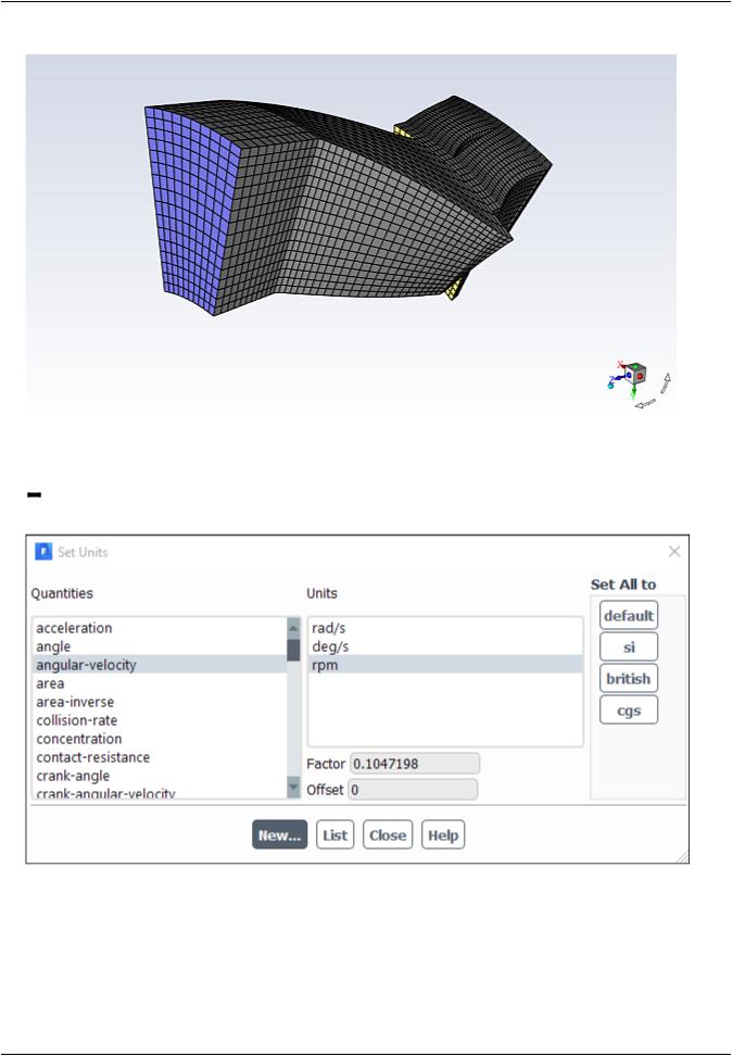
2.Examine the mesh (Figure 11.2: Rotor-Stator Display (p. 370)).
Orient the view to display the mesh as shown in Figure 11.2: Rotor-Stator Display (p. 370). The inlet of the rotor mesh is colored blue, the interface between the rotor and stator meshes is colored yellow, and the outlet of the stator mesh is colored red.
Release 2019 R1 - © ANSYS,Inc.All rights reserved.- Contains proprietary and confidential information |
|
of ANSYS, Inc. and its subsidiaries and affiliates. |
369 |
vk.com/club152685050Using Sliding Meshes | vk.com/id446425943
Figure 11.2: Rotor-Stator Display
3. Define the units for the model.


 Setup →
  General → Units...
a.Select angular-velocity from the Quantities selection list.
b.Select rpm from the Units selection list.
c.Select pressure from the Quantities selection list.
Scroll down the Quantities list to find pressure.
|
Release 2019 R1 - © ANSYS,Inc.All rights reserved.- Contains proprietary and confidential information |
370 |
of ANSYS, Inc. and its subsidiaries and affiliates. |

vk.com/club152685050 | vk.com/id446425943 |
Setup and Solution |
d.Select atm from the Units selection list.
e.Close the Set Units dialog box.
4.Use the text user interface to change zones rotor-per-1 and rotor-per-3 from wall zones to periodic zones.
a.Press Enter in the console to get the command prompt (>).
b.Type the commands as shown below in the console:
> mesh/modify-zones/list-zones |
|
|
|
|
id |
name |
type |
material |
kind |
---- |
------------------------- |
------------------ |
-------------------- |
---- |
13 |
fluid-rotor |
fluid |
air |
cell |
28 |
fluid-stator |
fluid |
air |
cell |
2 |
default-interior:0 |
interior |
|
face |
15 |
default-interior |
interior |
|
face |
3 |
rotor-hub |
wall |
air |
face |
4 |
rotor-shroud |
wall |
air |
face |
7 |
rotor-blade-1 |
wall |
air |
face |
8 |
rotor-blade-2 |
wall |
air |
face |
16 |
stator-hub |
wall |
air |
face |
17 |
stator-shroud |
wall |
air |
face |
20 |
stator-blade-1 |
wall |
air |
face |
21 |
stator-blade-2 |
wall |
air |
face |
22 |
stator-blade-3 |
wall |
air |
face |
23 |
stator-blade-4 |
wall |
air |
face |
5 |
rotor-inlet |
pressure-inlet |
|
face |
19 |
stator-outlet |
pressure-outlet |
|
face |
10 |
rotor-per-1 |
wall |
air |
face |
12 |
rotor-per-2 |
wall |
air |
face |
24 |
stator-per-2 |
wall |
air |
face |
26 |
stator-per-1 |
wall |
air |
face |
6 |
rotor-interface |
interface |
|
face |
18 |
stator-interface |
interface |
|
face |
11 |
rotor-per-4 |
wall |
air |
face |
9 |
rotor-per-3 |
wall |
air |
face |
25 |
stator-per-4 |
wall |
air |
face |
27 |
stator-per-3 |
wall |
air |
face |
/mesh/modify-zones> /mesh/modify-zones> make-periodic Periodic zone [()] 10
Shadow zone [()] 9
Rotational periodic? (if no, translational) [yes] yes Create periodic zones? [yes] yes
zone 9 deleted
created periodic zones.
5. Similarly, change the following wall zone pairs to periodic zones:
Zone Pairs |
Respective Zone IDs |
rotor-per-2 and rotor-per-4 |
12 and 11 |
stator-per-1 and stator-per-3 |
26 and 27 |
stator-per-2 and stator-per-4 |
24 and 25 |
Release 2019 R1 - © ANSYS,Inc.All rights reserved.- Contains proprietary and confidential information |
|
of ANSYS, Inc. and its subsidiaries and affiliates. |
371 |