vk.com/club152685050 | vk.com/id446425943

Chapter 12: Using Overset and Dynamic Meshes

This tutorial is divided into the following sections:

12.1.Prerequisites

12.2.Problem Description

12.3.Preparation

12.4.Mesh

12.5.Overset Interface Creation

12.6.Steady-State Case Setup

12.7.Unsteady Setup

12.8.Summary

The purpose of this tutorial is to provide guidelines and recommendations for setting up and solving

a dynamic overset mesh case. Overset mesh allows you to build up your case using multiple overlapping meshes that automatically get connected by interpolating cell data in the overlapping regions. The overset meshing technique is used in conjunction with the Six Degree of Freedom (6DOF) solver, allowing bodies to move as a result of fluid and/or external forces.

In this tutorial, you will learn:

•Reading and appending mesh files into the Fluent solver and establishing a flow domain with the overset approach from overlapping meshes.

•Best practices for overset mesh settings when two walls are close to each other or there is a very tight gap.

•Compiling the UDF to specify the properties of the pod.

•Setting up the moving zones and hooking the UDF.

•Running a steady-state calculation and continuing an unsteady calculation for the problem.

•Best practices for monitoring and diagnosing an overset case and postprocessing the results.

Note

Overset meshing has many applications beyond store separation. Refer to Overset Meshes in the Fluent User's Guide for additional information on overset meshing capabilities.

•ANSYS Fluent: Introduction to Overset Meshing

•ANSYS Fluent: Overset Meshing and Dynamic Meshes

•ANSYS Fluent: Using the Six Degrees of Freedom (Six DOF) Solver

vk.com/club152685050Using Overset and Dynamic| vkMeshes.com/id446425943

• ANSYS Fluent: Setting up a Dynamic Mesh Problem for a Piston and Reed Valve - Part 1

12.1. Prerequisites

This tutorial is focused on overset meshing and it assumes that you are familiar with the ANSYS Fluent interface and that you have a good understanding of the basic setup and solution procedures. Some of the basic steps in the setup and solution procedure will not be shown explicitly. In this tutorial, you will use the dynamic mesh model and the Six Degree of Freedom model. If you have not used these models before, refer to Section 10.6: Dynamic Meshes in the ANSYS Fluent User’s Guide. You will use a UDF to specify the properties of the pod. If you have not used UDFs before, refer to the Fluent Customization Manual.

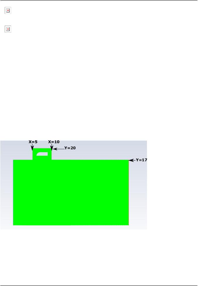
12.2. Problem Description

A rescue pod is dropped from a moving airplane flying at Mach 0.8. As the pod falls, it is subjected to pressure, viscous drag, and gravitational forces. These forces also create a moment on the pod, causing it to rotate about its center of gravity.

The pod is released from the aircraft at t=0.

Figure 12.1: Schematic of Problem

The representation of the problem is shown in Figure 12.1: Schematic of Problem (p. 408) A close view of the bay area and different walls with their interior zones are shown in Figure 12.2: Close View of Bay Area (p. 409).

Figure 12.2: Close View of Bay Area

12.3. Preparation

1.Download the overset_dynamic_mesh.zip file here.

2.Unzip overset_dynamic_mesh.zip to your working directory.

3.The mesh file overset-background-mesh.msh, Overset-component-mesh.msh, and the property.c can be found in the folder.

4.Use the Fluent Launcher to start the 2D version of ANSYS Fluent.

Fluent Launcher displays your Display Options preferences from the previous session.

For more information about Fluent Launcher, see starting ANSYS Fluent using the Fluent Launcher in the Fluent Getting Started Guide.

5.Ensure that the Display Mesh After Reading option is enabled.

6.Enable Double Precision.

7.Run in Parallel with 4 cores (specified under Processes).

12.4. Mesh

1.Read the mesh file Overset-background-mesh.msh.

File → Read → Mesh...

As ANSYS Fluent reads the mesh file, it will report the progress in the console. This mesh has three different zones that allow for a greater level of refinement where the pod will be falling and less refinement

vk.com/club152685050Using Overset and Dynamic| vkMeshes.com/id446425943

at the far field. Dividing the background mesh into multiple zones allows for non-conformal interfaces between the other zones that will not be in the overset interface.

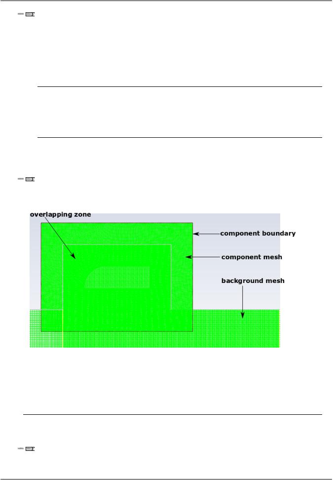
Note

Fluent uses the terminology of a component mesh and a background mesh. The mesh containing the moving object is called component mesh and stationary mesh is called the background mesh. The outer boundary of component mesh is referred as component boundary.

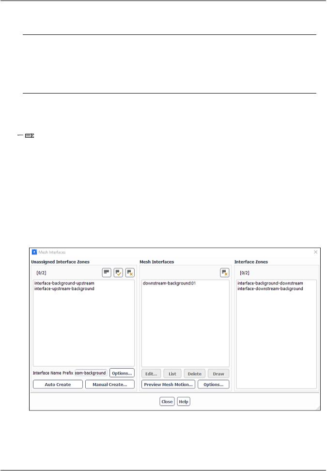
2.In this step you will create mesh interfaces between multiple zones in the stationary mesh. This mesh has three cell zonesupstream, downstream, and fluid-background.

Domain → Interfaces → Mesh...

a.Select interface-background-downstream and interface-downstream-background in the Unassigned Interface Zones list.

b.Enter downstream-background for Interface Name Prefix.

c.Click Auto Create.

d.Select interface-background-upstream and interface-upstream-background in the Unassigned Interface Zones list.

e.Enter upstream-background for Interface Name Prefix.

f. Click Auto Create and close the Mesh Interfaces dialog box.

3.Append the component mesh file

Domain → Zones → Append → Append Case File...

a.Select overset-component-mesh.msh and click OK.

b.Click OK in the Warning dialog box that appears stating that some zone IDs have changed.

c.If you have the Display Mesh After Reading option enabled in the Fluent Launcher, then you must refresh the graphics window by right-clicking in the graphics window and selecting Refresh Display.

Note

Fluent will append the component mesh and two meshes will overlap each other. If background and component meshes are present in the same mesh file, then you can start directly from the mesh file without appending.

4.Display the mesh.

Domain → Mesh → Display

a. Select all surfaces and click Display.

b.Close the Mesh Display dialog box.

Note

There are approximately 110 K mesh elements in this case.

5.Check the mesh.

Domain → Mesh → Check → Perform Mesh Check