vk.com/club152685050 | vk.com/id446425943Multi-Shot Ice Accretion with Automatic Mesh Displacement

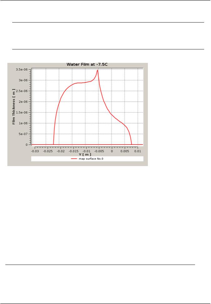
16.Leave the other default settings unchanged and click Calculate to update the 2D plot in the ChartViewer. The figure below shows the output of the macro.

Note

Users are invited to modify the input parameter of 2D-Plot (with) → Y-Axis to view different fields of the ICE3D solution.

Figure 27.26: 2D-Plot in CFD-Post, Water Film Distribution

27.6. Multi-Shot Ice Accretion with Automatic Mesh Displacement

As ice grows, the geometric profile of the contaminated airfoil changes which changes the flow of air and water droplets around it. The quasi-steady multishot approach allows simulation of realistic and accurate ice shapes. In this approach, the total time of ice accretion is divided into smaller steady-state intervals (shots), where the mesh used to calculate the airflow, the droplet impingement, and the ice accretion is updated at the end of each shot to account for the ice shape produced at each shot.

In the current version of Fluent Icing, multishot runs are done using automatic mesh displacement, where the ice surface is used to displace the contaminated walls and consequently the volume mesh around these walls. This process keeps the number of nodes and elements constant. As the ice shape grows, the total area covered by the boundary wall mesh increases which changes the size and the aspect ratio of the elements near the ice. This may result in a less than optimal grid spacing if the initial (undeformed) mesh is not fine enough. For complex ice shapes, manual remeshing maybe required in order to continue the multishot process when using automatic mesh displacement.

Note

FENSAP-ICE is able to utilize automatic remeshing in addition to the classic mesh deformation when simulating multi-shot icing. Remeshing of the iced surface refines and reorganizes the mesh topology on and around the ice, leading to more stable and ac-

vk.com/club152685050In-F ight Icing Tutorial Using| vk.Fluentcom/id446425943Icing

curate air and droplet solutions for the next shot. Negative volume elements that often form with large mesh deformations are also avoided with remeshing. These options are not yet supported by Fluent Icing. For more information regarding automatic remeshing, consult Automated Sequences and Multishot Icing Calculations within the FENSAP-ICE User Manual

1.Launch Fluent Icing from your working directory, FLUENT_ICING_NACA0012.

2.Go to File → Preferences…. Select Icing on the left hand-side of the Preferences window. Assign a number of CPUs, 2 to 4 CPUs, next to Default Fluent CPU and set Default work folder to the location of your working directory.

3.Go to File → Open case…. Browse to and select the file naca0012_rough_mvd_m7p5C.cas, created in Fluent Icing Ice Accretion on the NACA0012 (p. 912). In this tutorial, you will simulate 3 quasi-steady shots using the same in-flight icing conditions of the naca0012_rough_mvd_m7p5C.cas.

4.A message window will ask you to launch Fluent, click Yes. A new simulation tree appears under naca0012_rough_mvd_m7p5C.cas(loaded) in the Outline View window. All airflow, droplet and ice conditions and solutions previously configured and computed in the previous simulation are automatically imported under that .CAS.

5.Go to Set-up → Ice and its Properties window and check Beading under Model. Beading is the roughness model of the Ice component. At the end of each shot, Beading will produce a roughness distribution that is used by the airflow solver (Fluent or FENSAP (beta)) during the next shot. This approach removes any arbitrary specification of roughness value and removes empiricism in the specification of roughness. The first shot always needs some initial roughness, 0.5 mm in Flow Solution on the Rough NACA0012 Air-

foil (p. 892), since Ice is not run a priori. However, the remaining shots will use the distribution obtained from the beading model.

Note

Alternatively, the initial shots could be conducted over small time intervals where the surface roughness can be allowed to grow from 0 to a reasonable level, removing the need to specify an initial roughness value. For internal flows, it is not recommended to start with a non-zero initial roughness instead. Roughness should be allowed to build progressively using shorter icing shots.

6.Click on Solve and, in its Properties window, under Multi-shot:

•Set Number of shots to 3

•Check Save files at each shot to examine the steady-state solutions at the end of each shot.

7.Under Solve → Ice,

•In Time, change the Total time of ice accretion [s] from 420 to 140 which corresponds to 1/3rd of the total time.

vk.com/club152685050 | vk.com/id446425943Multi-Shot Ice Accretion with Automatic Mesh Displacement

• In Output, check Run grid displacement to update the grid at the end of each shot.

Note

As the grid quality may deteriorate after each shot, it might be necessary to change several settings in Solve to improve the robustness and convergence of these simulations. In this manner, the number of iterations can be increased for Airflow and Particles and the CFL number can be lowered in the case of Particles.

8.Right-click Ice under Solve and choose Reset to erase the solution of the previous one shot simulation.

9.Go to File → Save Case as …, and name it naca0012_rough_mvd_m7p5C_multi. All multishot solutions will start with this name followed by the shot number and a suffix that describes the nature of the output file.

10.Launch the multishot calculation by right-clicking Solve and then by selecting Run multishot.

11.Once all the computations are complete, go to Ribbon menu and select View. In Quick-view, click Ice cover → Multishot ice cover - Viewmerical to see the final ice shape of the multishot calculation.

Figure 27.27: 3-Shots Ice Shape at -7.5 C

12.Compare the ice shape of the multishot run to that of the single shot run while the Viewmerical window that displays the multi-shot ice shape is up.

13.In the Objects panel, rename this object by double-clicking on its original name in the Object window and enter -7.5C, 3 shots in the window Rename dataset.

14.Click on the button located at the right corner of the Object panel. A window appears to load a pair of files, a grid file and its solution file.

vk.com/club152685050In-F ight Icing Tutorial Using| vk.Fluentcom/id446425943Icing

15.Click on the folder icon of Grid file and select the naca0012_rough_mvd_m7p5C.ice.grid file located inside your working directory.

16.Press the Load button. A new data set is added to the Object panel. Rename this dataset by double-clicking on its original name and enter -7.5C, 1 shot in the window Rename dataset.

17.Click the lock icon at the lower right of the data set list in the Objects window.

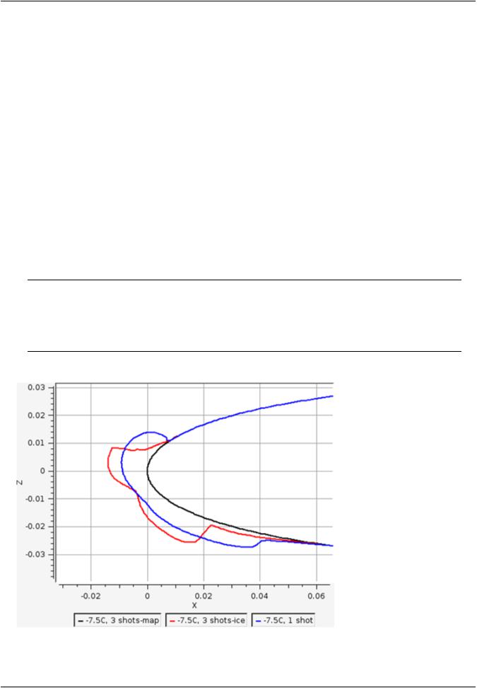
18.Go to the Query panel and activate the 2D plot. Set the Mode to Geometry and Cutting plane to Z. Set the horizontal axis to X. The three curves showing NACA0012 and the ice shapes should be visible. Change the curve colors and thickness using the Curve Settings in the cube menu located at the top right. You can also draw a zoom box by Shift + left-click.

Note

The multishot simulation produces an upper horn that is more pronounced due to higher water droplet catch area and higher heat fluxes with increase in curvature. The lower part of the ice is also thicker where the roughness has grown beyond the initial 0.5mm to about 1mm (average), which causes the water film to freeze sooner and show less runback compared to the single shot solution.

Note

The curves that have the -map suffix refer to the original surface and the curves that have the -ice suffix refer to the final iced surface (at 420 s).

Figure 27.28: Ice Shapes at -7.5 C, Obtained Using One Shot and Three Shots Computations