vk.com/club152685050 | vk.com/id446425943Postprocessing an Ice Accretion Solution Using CFD-Post Macros

The film height and extent grow with increasing icing temperatures. At -25 °C, all droplets freeze upon impact and there is no water film and runback on the surface, producing a rime ice shape. In the contrary, the amount of film and water runback of the other two cases clearly produce ice horns and form glaze ice shapes.

40. Do not close this Fluent Icing session if you would like to proceed to the next section.

27.5. Postprocessing an Ice Accretion Solution Using CFD-Post Macros

In this tutorial, you will learn how to quickly post-process one-shot Ice results (Ice shape and ice solution fields) using two dedicated CFD-Post macros: Ice Cover – 3D-View and Ice Cover – 2D-Plot. For this purpose, the icing solution of your icing simulation at -7.5 °C of Fluent Icing Ice Accretion on the NACA0012 (p. 912) is used and, therefore, completion of Fluent Icing Ice Accretion on the

NACA0012 (p. 912) is required.

For more information regarding these macros, consult CFD-Post Macros within the FENSAP-ICE User Manual.

1.Inside your Fluent Icing window, go to Ribbon menu and select View. In Quick-view, click Ice cover → Ice cover – CFD-Post.

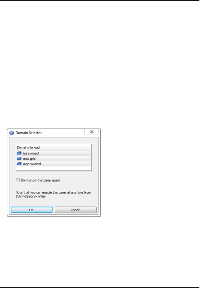
2.After opening CFD-Post, a Domain Selector window will request confirmation to load the following domains: ice swimsol, map grid, and map swimsol. Click OK to proceed.

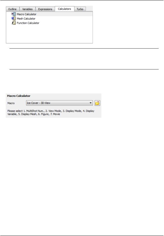
3.Go to the Calculators tab and double-click on Macro Calculator. The Macro Calculator’s interface panel will be activated and displayed.

vk.com/club152685050In-F ight Icing Tutorial Using| vk.Fluentcom/id446425943Icing

Note

The Macro Calculator can also be accessed by selecting Tools → Macro Calculator from the CFD-Post’s main menu.

4.Select the Ice Cover – 3D-View macro script from the Macro drop-down list. This will bring up the user interface which contains all input parameters required to view ICE3D output solutions in the CFD-Post 3D Viewer.

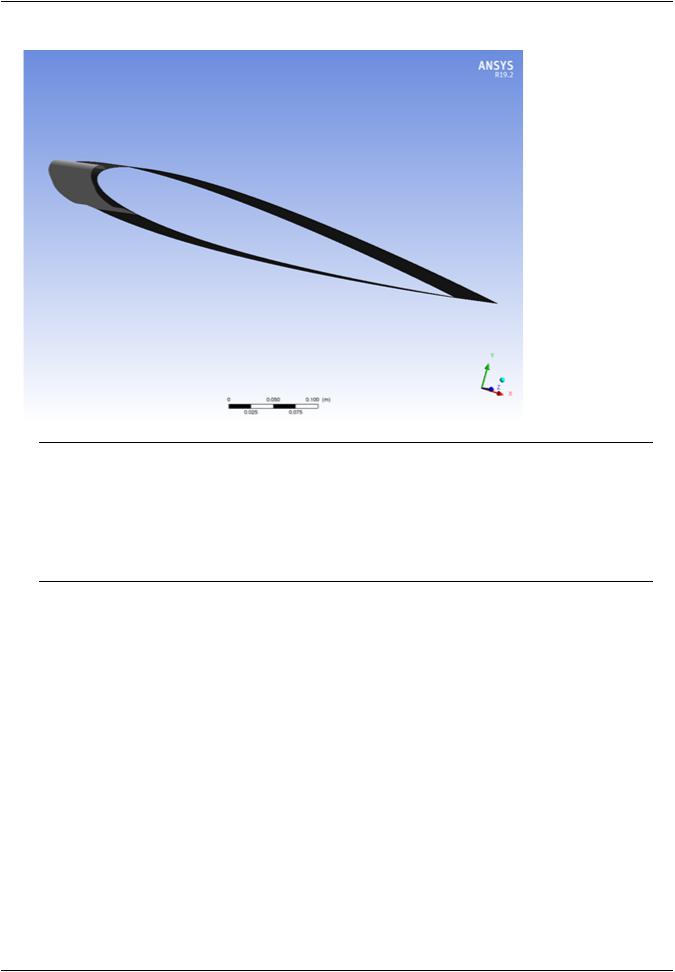
5.The default settings inside the Macro Calculator panel will allow you to automatically output the ice shape of a one-shot icing simulation by pressing Calculate. The figure below shows the output of the default settings of the macro.

vk.com/club152685050 | vk.com/id446425943Postprocessing an Ice Accretion Solution Using CFD-Post Macros

Figure 27.22: Ice View with CFD-Post, Ice Cover

Note

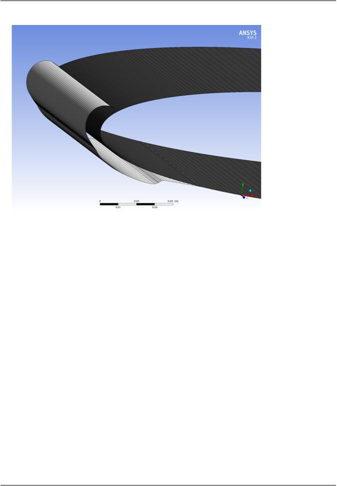
To change the style of the ice shape display, go to Display Mode and select one of following options: Ice Cover, Ice Cover – Shaded, Ice Cover (only) or Ice Cover (only) - shaded. To output the surface mesh of the ice shape, go to Display Mesh and select Yes. The figure below shows the output of activating Ice Cover under Display Mode and of selecting Yes under Display Mesh.

vk.com/club152685050In-F ight Icing Tutorial Using| vk.Fluentcom/id446425943Icing

Figure 27.23: Ice View in CFD-Post, Ice Cover with Display Mesh

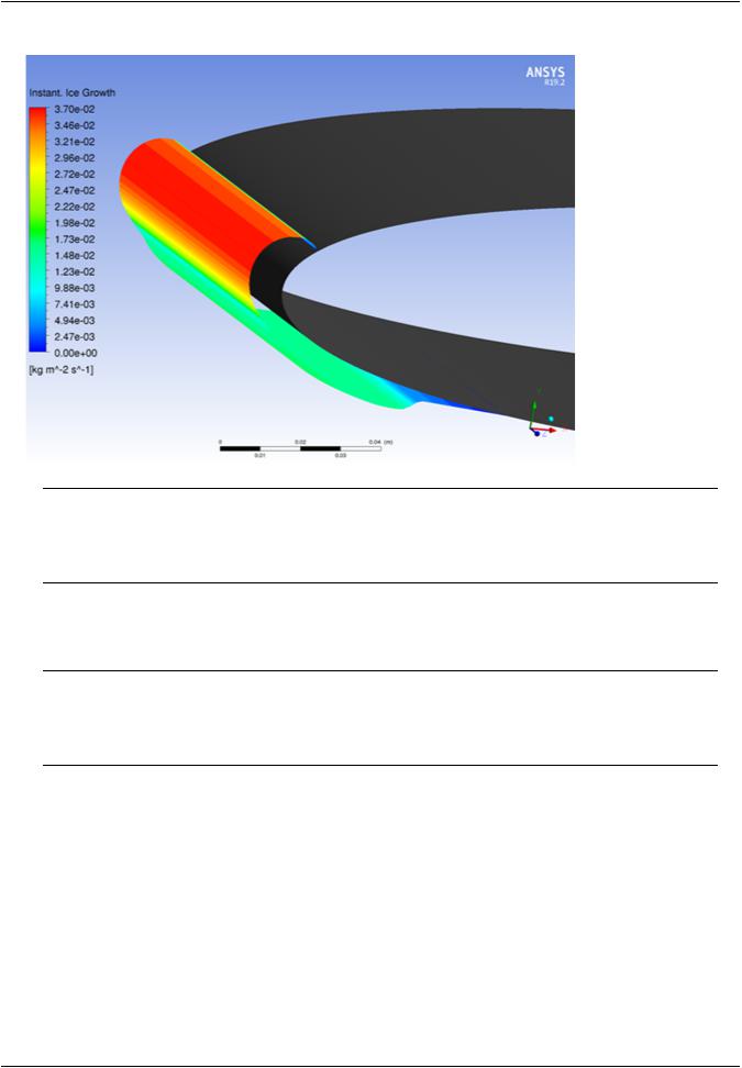
6.To display the solution fields of your icing simulation, you can either select Ice Solution – Overlay, Ice Solution or Surface Solution under Display Mode. In this case, you will output the ice accretion rate over the ice layer. To do this, select Ice Solution – Overlay in Display Mode, Instant. Ice Growth (kg s^-1 m^- 2) in Display Variable and No in Display Mesh to turn off the displaying surface mesh.

7.Click Calculate to view the instantaneous ice growth over the ice shape. The figure below shows the output of the macro.

vk.com/club152685050 | vk.com/id446425943Postprocessing an Ice Accretion Solution Using CFD-Post Macros

Figure 27.24: Ice View in CFD-Post, Instantaneous Ice Growth over Ice Cover Surface

Note

Users are invited to modify the input parameter of Display Variable to view different fields of the ICE3D solution.

8.You will now explore some quick post-processing capabilities of the Ice Cover – 2D-Plot macro. In the Macro drop-down list of the Macro Calculator panel, change the macro to Ice Cover – 2D-Plot.

Note

This switches the macro from Ice Cover – 3D-View to Ice over – 2D-Plot. Switch back to Ice Cover – 3D-View in the same way if needed.

9.Change Plot’s Title from default, ICE SHAPE PLOT, to Ice Shape at -7.5 C, since you will be first creating a 2D-plot of the ice shape.

10.Inside 2D-Plot (with),

• Set Mode to Geometry to output an ice shape. The other options output the ice solution fields.

•Set Cutting Plane to Z plane. Specify a Z=0 plane by setting X/Y/Z Plane to 0.

•Set the X-Axis to X and the Y-Axis to Y.

11.To center the 2D-Plot around the leading edge of the NACA0012, in 2D-Plot (with),

vk.com/club152685050In-F ight Icing Tutorial Using| vk.Fluentcom/id446425943Icing

•Change the (x)Range of the X-Axis from Global to User Specified. Specify values of 0.075 and -0.01 in the input boxes of (Usr.Specif.x)Max and (Usr.Specif.x)Min, respectively.

•Change the (y)Range of the Y-Axis from Global to User Specified. Specify values of 0.03 and -0.03 in the input boxes of (Usr.Specif.y)Max and (Usr.Specif.y)Min, respectively.

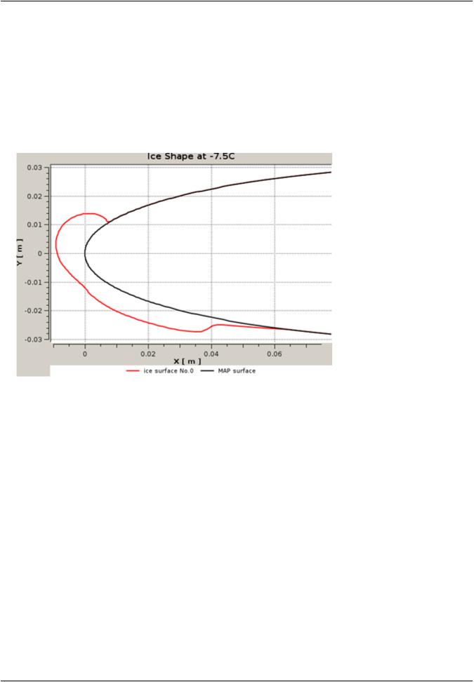
12.Leave the other default settings unchanged and click Calculate to create a 2D-Plot of the ice shape in a floating ChartViewer of CFD-Post. Adjust the output window’s size. The figure below shows the output of the macro.

Figure 27.25: 2D-Plot in CFD-Post, Clean Wall Surface and Ice Cover Surface

13. To create a 2D-plot of an ice solution field, first change the name of the plot. In this case, enter Water Film at -7.5 C in the Plot’s Title field since you will create a water film 2D plot along the thickness of the airfoil.

14.Inside 2D-Plot (with),

•Set Mode to Solution (on Map Surfaces) to output the water film over the NACA0012. Selecting Solution (on Ice Surfaces) will output the ice field over the ice shape.

•Set Cutting Plane to Z plane. Specify a Z=0 plane by setting X/Y/Z Plane to 0.

•Set the X-Axis to Y.

•Set the Y-Axis to Film Thickness (m).

15.To center the 2D-Plot around a meaningful scale to clearly see the water film distribution, in 2D-Plot (with),

•Make sure that (x)Range of the X-Axis is set to User Specified. Enter values of 0.01 and -0.03 for

(Usr.Specif.x)Max and (Usr.Specif.x)Min, respectively.

•Set (y)Range of the Y-Axis to Global. The macro will use the max./min. values of the water film thickness to define the range of the Y-axis.