vk.com/club152685050 | vk.com/id446425943

Chapter 27: In-Flight Icing Tutorial Using Fluent Icing

27.1. Fluent Airflow on the NACA0012 Airfoil

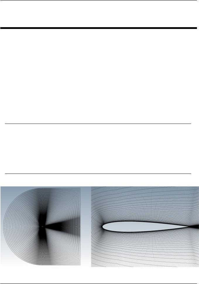
The objective of this tutorial is to obtain an airflow solution around a rough NACA0012 airfoil using Fluent, within the Fluent Icing framework, and to use this solution for water catch and ice accretion simulations. The NACA0012 grid corresponds to the case file produced at the end of Flow Solution on the Clean NACA0012 Airfoil within the FENSAP-ICE Tutorial Guide. The computational grid consists of 114,700 nodes and 56,810 hexahedral cells. Symmetry conditions are imposed on each spanwise boundary of the grid. The airfoil chord length is 0.5334 meters (21 inches) and the depth of elements along the span (Z-direction) is 0.1 meters. A no-slip wall boundary is imposed on the airfoil surface. Since the flow is viscous and turbulent, grid points have been clustered around the airfoil to better capture the boundary layer and wake. The initial cell height is 2.5e-6 chords, set up such that the maximum Y+ is below 1 in the first layer, and the expansion ratio is 1.14 in the normal direction which is a fine-grid setting that is required for capturing boundary layers. Far-field conditions are imposed on the outer surface of the grid. The mesh density can be considered medium.

Note

This tutorial uses the same in-flight conditions as In-Flight Icing using FLUENT within FENSAPICE within the FENSAP-ICE Tutorial Guide.

FENSAP-ICE modules used in Fluent Icing solve 2-D problems using a volume mesh of a single layer of 3-D elements instead of surfaces, for generalized implementation of the governing equations. This requires Fluent to be executed in 3-D mode even if the computational domain is in fact 2-D.

Figure 27.1: NACA0012 Structured C-Mesh Overview and Close-Up

vk.com/club152685050In-F ight Icing Tutorial Using| vk.Fluentcom/id446425943Icing

For more information on how to set up the input parameters of Fluent for in-flight icing simulations, you are invited to read Recommendations to Set up a Fluent Calculation within the FENSAP-ICE User Manual or the Recommended settings section under Fluent Icing within the Fluent User's Guide.

27.2. Flow Solution on the Rough NACA0012 Airfoil

Ice forms surface roughness where it accretes. This roughness increases the momentum deficit and skin friction, which in turn thickens the boundary layer and increases drag. Convective heat flux is also increased through additional turbulent conductivity within the boundary layer. It is therefore essential

to properly model the roughness produced naturally by the ice accretion process to obtain realistic ice shapes. Fluent Icing can model sand-grain roughness by means of modifying the wall turbulence model boundary conditions and eventually increasing the intensity of the eddy (turbulent) viscosity in

the boundary layer. The micro scale roughness is usually in the range of 0.1 ~ 3.0 mm. It can be specified on each wall as a constant value, or as a distribution via empirical or analytical methods. Roughness value greatly influences the final ice shape; therefore, it must be chosen appropriately. See Surface Roughness within the FENSAP-ICE User Manual or Set-up → Boundary Conditions → Wall and Set-up → Ice under Fluent Icing within the Fluent User's Guide for more details on surface roughness.

Download the FLUENT_ICING.zip file here.

1.Create a working directory folder and name it FLUENT_ICING_NACA0012.

2.Go to file ../workshop_input_files/Input_Grid/Naca0012/naca0012.clean.cas. Copy this case file along with its data file (naca0012.clean.dat) into your working directory FLUENT_ICING_NACA0012.

This case contains all the proper airflow settings required to conduct in-flight icing simulations using the following flight condition. See Flow Solution on the Clean NACA0012 Airfoil within the FENSAPICE Tutorial Guide for more detail.

3.Table 27.1: Flight Condition Table

In this tutorial, only the wall boundaries require set-up as the original .CAS file corresponds to a clean surface.

4.Launch Fluent Icing from your working directory.

5.Go to File → Preferences…. Select Icing on the left hand-side of the Preferences window. Assign a number of CPUs, 2 to 4 CPUs, next to Default Fluent CPU, check Define working directory and set Working directory to the location of your working directory. Click Ok. A message box that asks you to confirm your changes appears. Press Yes.

6.Go to File → Open Case, and browse to and select the file naca0012.clean.cas located in your working directory.

7.A message window will ask you to import the data file and then to launch Fluent, click Yes in both cases. In your Fluent Icing window, a new simulation tree appears under naca0012_clean.cas (loaded) in the

Outline View window.

8.Select Set-up under naca0012_clean.cas (loaded) and, in its Properties window, uncheck Particles and Ice.

9.Inside the Outline View window, right on the Airflow icon located under Set-up and select Update with Fluent Case settings to make sure that the Fluent simulation settings are properly transferred to Fluent Icing.

10.Under Set-up → Airflow, check Sync. with Fluent ref. conditions to synchronize the Properties of Airflow panel with the Reference Values panel of Fluent.

11.Under Set-up → Boundary Conditions, update the following wall surfaces:

•Select the wall-5 boundary. In the Wall roughness section of the Airflow panel, select High roughness for icing and set its Roughness Height (m) to 0.0005 m.

•Repeat this process for wall boundaries wall-6, wall-7, and wall-8.

12.Under Solve, right-click Airflow from the side menu. Select Initialize. A Hybrid initialization is executed using the settings of the original case file.

13.Under Solve → Airflow, increase the Number of iterations to 1000. A steady state simulation will be executed since the original case file contains steady state settings.

Note

Transient calculations are not yet supported. Therefore, the original case file must contain

asteady state set-up.

14.Right-click the Airflow icon under Solve and select Calculate to launch this simulation.

15.Once the simulation is complete, go to File → Save Case as… and save this calculation in the project directory FLUENT_ICING_NACA0012. Name this simulation naca0012_rough.

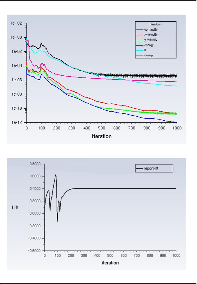
16.Take a look at the convergence history of this simulation in the Graphics window located at the right of your screen. The following two figures show the convergence of residuals and lift and drag coefficients. You can enlarge and move the legend box in the Graphics windows by dragging one side of or whole the box.

In the console, the residuals and coefficients are provided at each iteration. As it is not possible to zoom in on the graphs, the printed values in the log can be referred to if needed. Examine the convergence of lift and drag coefficients listed as “report-lif” and “report-dra”. Lift and drag coefficients have converged to 0.40367 and 0.019842 respectively.

vk.com/club152685050In-F ight Icing Tutorial Using| vk.Fluentcom/id446425943Icing

Figure 27.2: Scaled Residuals

Figure 27.3: Convergence of Lift and Drag Coefficients of the Rough Airfoil