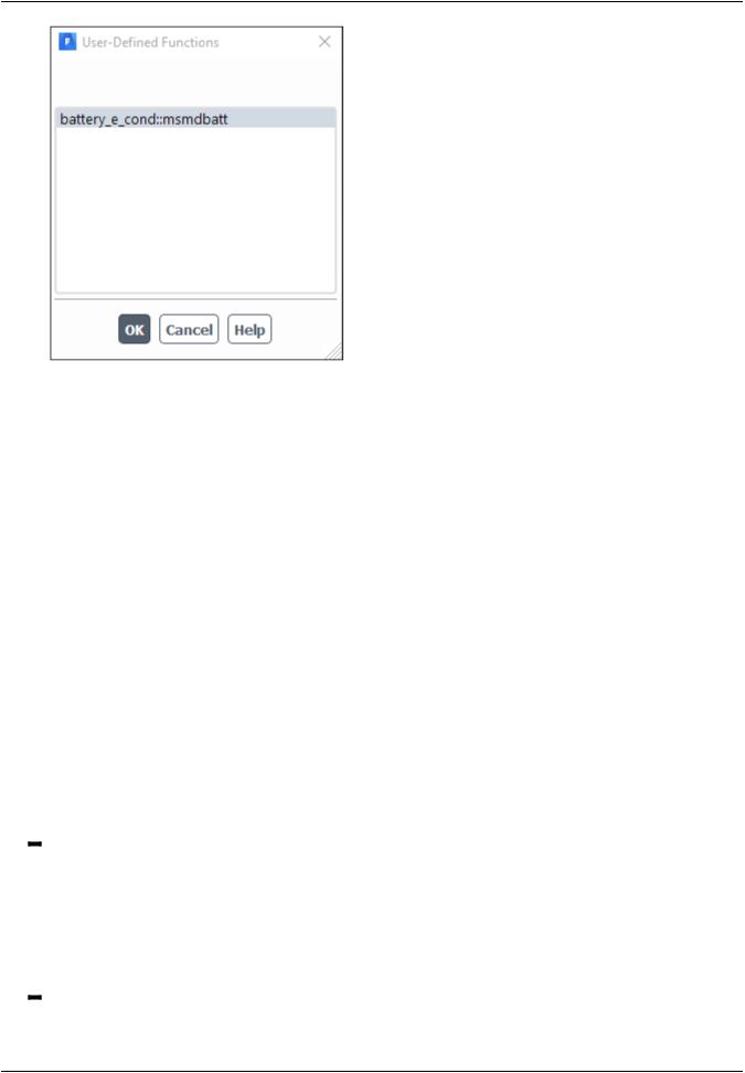
d.In the Question dialog box, click No to retain e-material and add the new busbar_material material to the materials list.

Fluent hooks the battery_e_cond::msmdbatt UDF to the busbar material.

e.Close the Create/Edit Materials dialog box.

f.Edit the busbar_material material and ensure that busbar_material (bus) is selected from the

Fluent Solid Materials drop-down list.

g.Set Thermal Conductivity to 20.

h.Retain the default value of 3.541 e7 [1/ohm-m] for Electrical Conductivity.

i.Click Change/Create.

j.Close the Create/Edit Materials dialog box.

26.4.4.3. Defining Cell Zone Conditions

Assign e_material to all the cell zones and busbar_material to all the tabs and busbars. 1. Assign e_material to the cell_1 cell zone.

Setup → Cell Zone Conditions → cell_1 → Edit...

a.In the Solid dialog box, select e_material from the Material Name drop-down list.

b.Click OK.

2.Copy the cell zone condition for the cell_1 zone to the cell_2 and cell_3 cell zones.

Setup → Cell Zone Conditions → cell_1 → Copy...

vk.com/club152685050Simulating a 1P3S Battery| vkPack.com/id446425943Using the MSMD Battery Model

a.In the Copy Conditions dialog box, select cell_1 in the From Cell Zone list.

b.In the To Cell Zones list, select cell_2 and cell_3.

c.Click Copy.

d.Click OK in the Question dialog box to copy the cell zone conditions and close the Copy Conditions dialog box.

3.In a similar manner, assign busbar_material to all the tabs and busbars cell zones.

26.4.4.4. Defining Boundary Conditions

Define the thermal boundary conditions for all walls for the cells, busbars, and tabs. The boundary conditions for the two UDSs have been set automatically when you defined the cell zone conditions.

1.Set the convection boundary condition for wall-cell_1.

Physics → Zones → Boundaries

a.In the Boundary Conditions task page, double-click wall-cell_1.

b.In the Wall dialog box, under the Thermal tab, configure the following settings:

i.Under Thermal Conditions, enable Convection.

ii.Set Heat Transfer Coefficient to 5 [w/m2K].

iii.Set Free Stream Temperature to 300 [K].

iv.Click OK to close the Wall dialog box.

2.Copy the boundary conditions for wall-cell_1 to wall-cell_2, wall-cell_3 and all the tab and busbar wall zones (a boundary zones that have names starting with the "wall" string and containing the "bar" or "tabzone" string).

Setup → Boudnary Conditions → wall-cell_1 → Copy...

26.4.4.5. Specifying Solution Settings

1.Turn off the flow equation.

Solution → Controls → Equations...

a.In the Equations dialog box, deselect Flow from the Equation selection list.

b.Click OK.

2.Remove the convergence criteria to ensure that automatic convergence checking does not occur.

Solution → Reports → Residuals...

a.In the Residual Monitors dialog box, select none from the Convergence Criterion drop-down list.

b.Click OK.

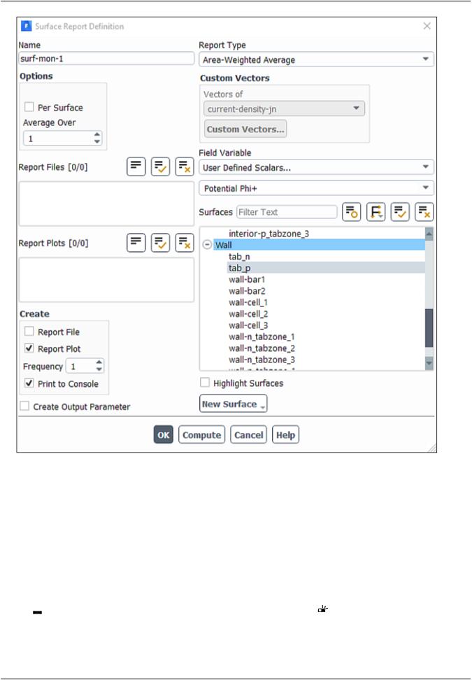
3.Create a surface report definition for the voltage at the positive tab.

Solution → Reports → Definitions → New → Surface Report → Area-Weighted Average

vk.com/club152685050Simulating a 1P3S Battery| vkPack.com/id446425943Using the MSMD Battery Model

a.In the Surface Report Definition dialog box, enter surf-mon-1 for Name.

b.Select User Defined Scalars... and Potential Phi+ from the Field Variable drop-down lists.

c.From the Surfaces selection list, select tab_p.

d.In the Create group box, enable Report Plot and Print to Console.

e.Click OK to save the surface report definition and close the Surface Report Definition dialog box.

f.Modify the attributes of the plot axes.

Solution → Monitors → Report Plots → surf-mon-1-rplot Edit...

i.In the Edit Report Plot dialog box, under the Plot Window group box, click the Axes... button to open the Axes dialog box.

ii.Select the X axis and set Precision to 0.

iii.Click Apply.

iv.Select the Y axis and set Precision to 2.

v.Click Apply and close the Axes dialog box.

Note

You must click Apply to save the modified settings for each axis.

vi. Click OK

g.Ensure that time-step is selected from the Get Data Every drop-down list.

h.Click OK.

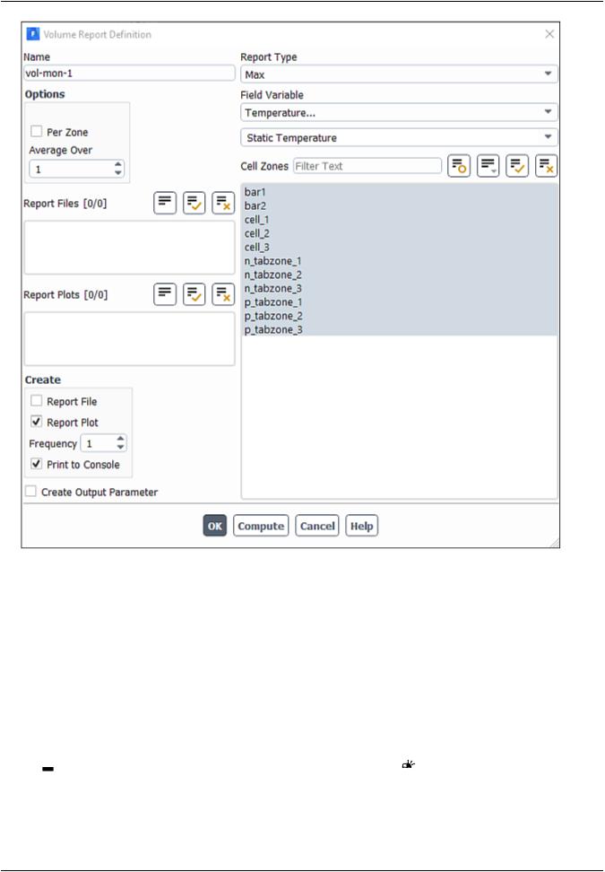
4.Create a volume report definition to monitor the maximum temperature in the domain.

Solution → Reports → Definitions → New → Volume Report → Max...

vk.com/club152685050Simulating a 1P3S Battery| vkPack.com/id446425943Using the MSMD Battery Model

a.In the Volume Report Definition dialog box, enter vol-mon-1 for Name.

b.Select Temperature... and Static Temperature from the Field Variable drop-down lists.

c.From the Cell Zones selection list, select all zones.

d.In the Create group box, enable Report Plot and Print to Console.

e.Click OK to save the volume report definition settings and close the Volume Report Definition dialog box.

f.Modify the attributes of the plot axes.

Solution → Monitors → Report Plots → vol-mon-1-rplot Edit...

i.In the Edit Report Plot dialog box, under the Plot Window group box, click the Axes... button to open the Axes dialog box.