Number of battery series stages =1; Number of batteries in parallel per series stage=1

****************END OF BATTERY CONNECTION INFO**************

g.Verify that the connection information is correct.

h.Click OK to close the MSMD Battery Model dialog box.

In the background, Fluent automatically hooks all the necessary UDFs for the problem.

i.Click OK to close the Information dialog box.

25.4.4.2. Defining New Materials for Cell and Tabs

Define the new e_material material for the battery’s cell, p_material for the positive tab, and n_material for the negative tab.

In the battery model, two user defined scalars, uds0 and uds1, are solved for the positive and negative potentials, respectively. To specify the electric conductivity of the active material you need to define the UDS diffusivity.

Important

For the battery active material, you must define the electric conductivity via the UDS diffusivity on a per-scalar basis. ANSYS Fluent will use these two UDS scalars to solve the differential equations; for details, see the Fluent Advanced Add-On Modules documentation.

For the battery passive conductive zones, such as tabs or busbars, you must define the UDS diffusivity using a user-defined function (UDF) and define the material’s electric conductivity using the Electrical Conductivity entry field.

1.Create the electric material.

Physics → Materials → Create/Edit...

vk.com/club152685050Simulating a Single Battery| vkCell.com/id446425943Using the MSMD Battery Model

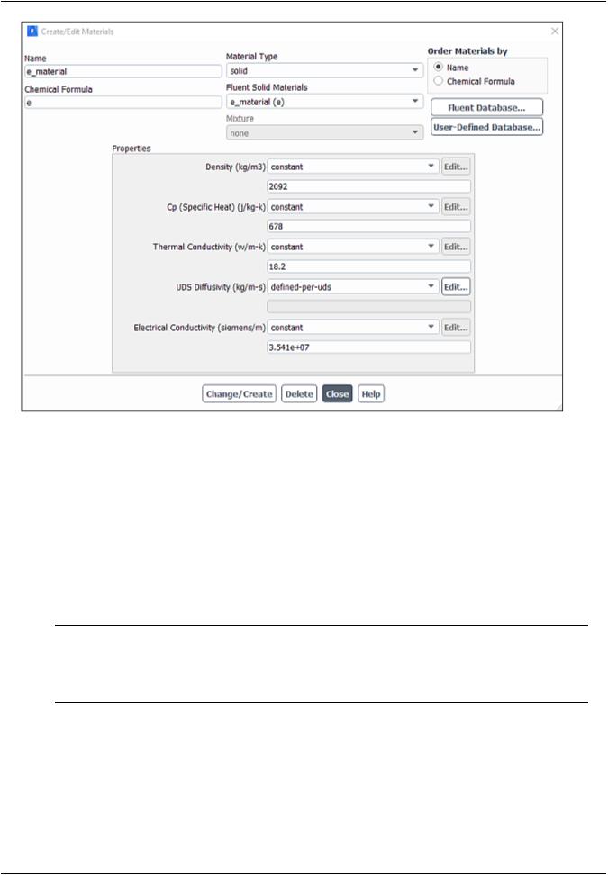
a.In the Create/Edit Materials dialog box, select solid from the Material Type drop-down list.

b.Enter e_material for Name and e for Chemical Formula.

c.Under Properties, set Density to 2092 [kg/m3].

d.Set CP (Specific Heat) to 678 [J/kg-K].

e.Set Thermal Conductivity to 18.2 [W/m-K].

f.Ensure that define-per-uds is selected from the UDS Diffusivity drop-down list and click Edit... next to UDS Diffusivity.

Note

If the UDS Diffusion Coefficients are defined through the defined-per-uds option, the Fluent solver does not use the value for Electrical Conductivity.

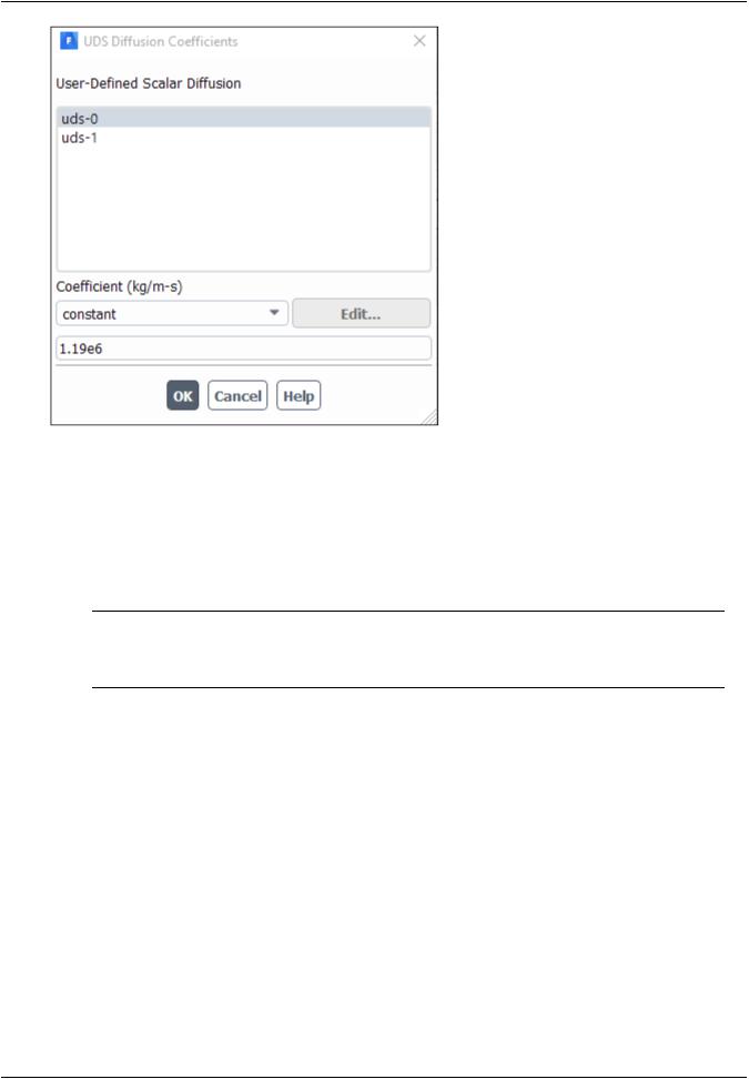
g. In the UDS Diffusion Coefficients dialog box, specify the user-defined scalars.

i.Select uds-0 in the User-Defined Scalar Diffusion list.

ii.Retain constant from the Coefficient drop-down list.

iii.Set Coefficient to 1.19e6 [1/ohm-m].

iv.In a similar way, set uds-1 to 9.83e5 [1/ohm-m] and close the UDS Diffusion Coefficients dialog box.

Note

The units for UDS Diffusivity are 1/ohm-m, and cannot be modified.

v.In the Question dialog box, click No to retain aluminum and add the new material (e_material) to the materials list.

Note

Refer to Appendix (p. 859) for information on how to calculate the battery cell property values.

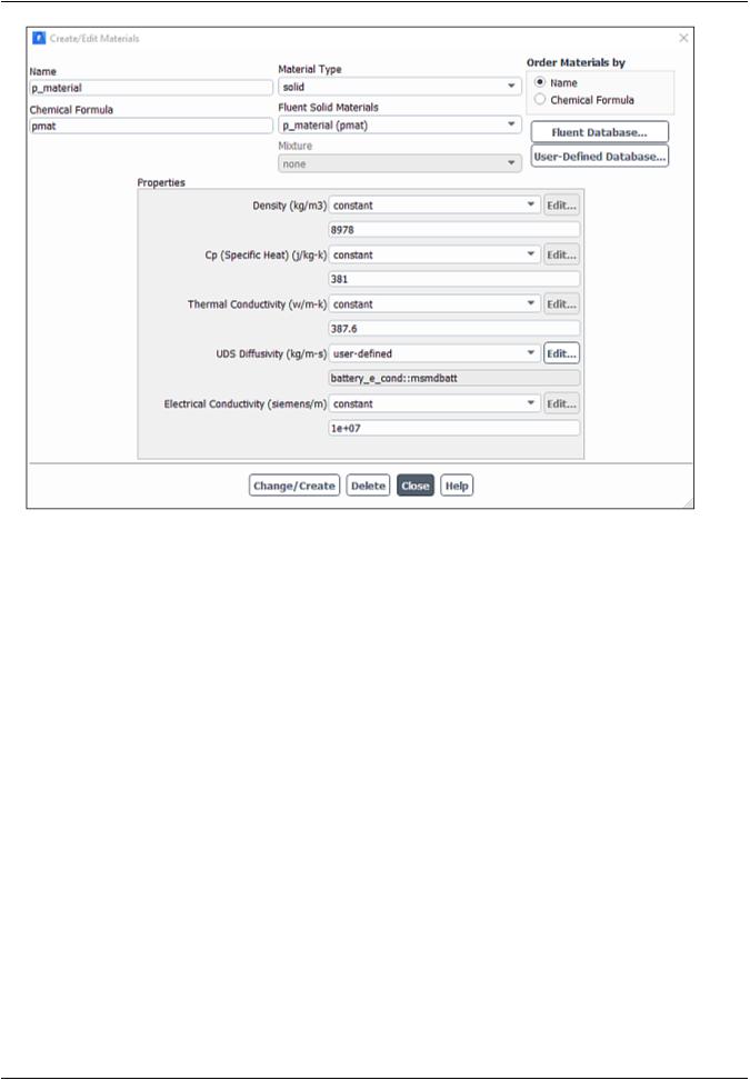
2. Create a new material for the positive tab by modifying copper from the solid material database.

vk.com/club152685050Simulating a Single Battery| vkCell.com/id446425943Using the MSMD Battery Model

The UDS Diffusivity for tab materials must be defined through the UDF as described below.

a.In the Create/Edit Materials dialog box, click Fluent Database....

b.In the Fluent Database Materials dialog box, make sure that solid is selected for Material Type.

c.Select copper from Fluent Solids Materials and click Copy and then Close.

The Create/Edit Materials dialog box now displays the copied properties for copper.

d.Enter p_material for Name and pmat for Chemical Formula.

e.Set the Electrical Conductivity to 1.0e7 [1/ohm-m].

f.Under Properties, select user-defined from the UDS Diffusivity drop-down list.

g.In the User-Defined Functions dialog box that opens, verify that battery_e_cond::msmdbatt is selected and click OK.