vk.com/club152685050Fluid Flow and Heat Transfer| vk.incom/id446425943a Mixing Elbow

b.Click OK to save the files and close the Select File dialog box.

c.Click OK to overwrite the files that you had saved earlier.

2.4.8. Adapting the Mesh

For the first run of this tutorial, you have solved the elbow problem using a fairly coarse mesh. The elbow solution can be improved further by refining the mesh to better resolve the flow details. ANSYS Fluent provides a built-in capability to easily adapt (locally refine) the mesh according to solution gradients.

In the following steps you will adapt the mesh based on the temperature gradients in the current solution and compare the results with the previous results.

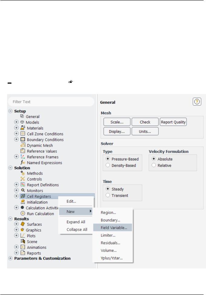
1.Define Cell Registers to Adapt the mesh in the regions of high temperature gradient.

Solution → Cell Registers New → Field Variable...

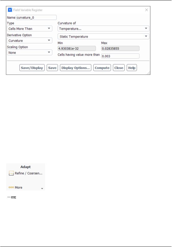
a.Select Cells More Than from the Type drop-down list.

b.Select Curvature from the Deriviative Option drop-down list.

c.Select Temperature... and Static Temperature from the Curvature of drop-down list.

d.Click Compute.

ANSYS Fluent will update the Min and Max values to show the minimum and maximum temperature gradient.

e.Enter a value of 0.003 for the Cells having value more than.

A general rule is to use 10% of the maximum gradient when setting the value for refinement.

f.Click Save and close the Field Variable Register daialog box.

2.Setup mesh adaption using the Cell Registers. For this task, you will use the Adapt group box in the Domain ribbon tab.

Domain → Adapt → Refine / Coarsen...

vk.com/club152685050Fluid Flow and Heat Transfer| vk.incom/id446425943a Mixing Elbow

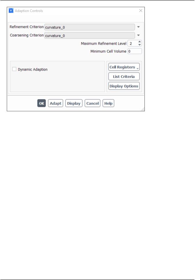
a.Select the previously defined curvature_0 cell register from the Refinement Criterion and Coarsening Criterion drop down lists.

ANSYS Fluent will not coarsen beyond the original mesh for a 3D mesh. Hence, it is not necessary to select the Coarsening Criterion in this instance.

b.Click Adapt.

c.Click Display.

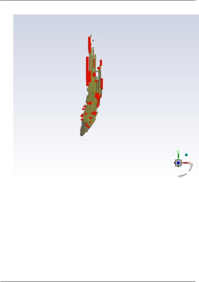
ANSYS Fluent will display the cells marked for adaption in the graphics window (Figure 2.12: Cells Marked for Adaption (p. 83)).

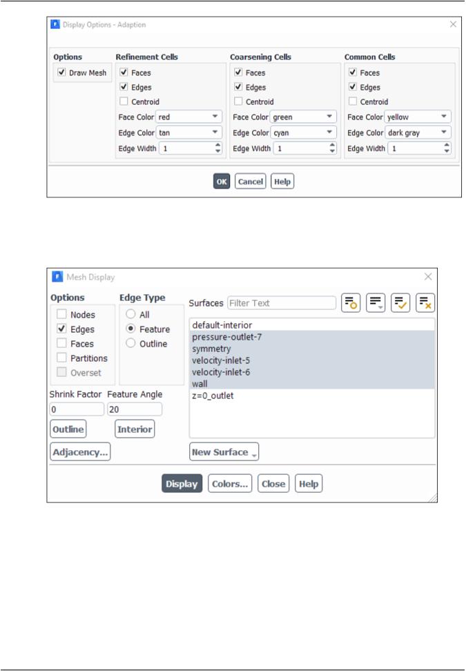
Extra You can change the way ANSYS Fluent displays cells marked for adaption (Figure 2.13: Al- ternative Display of Cells Marked for Adaption (p. 85)) by performing the following steps:

i.Click Display Options... in the Adaption Controls dialog box to open the Display Options - Adaption dialog box.

vk.com/club152685050Fluid Flow and Heat Transfer| vk.incom/id446425943a Mixing Elbow

ii.Enable Draw Mesh in the Options group box.

The Mesh Display dialog box will open.

iii.Ensure that only the Edges option is enabled in the Options group box.

iv.Select Feature from the Edge Type list.

v.Select all of the items except default-interior and z=0_outlet from the Surfaces selection list.

vi.Click Display and close the Mesh Display dialog box.

vii.Click OK to close the Display Options - Adaption dialog box.

viii.Click Display in the Adaption Controls dialog box.

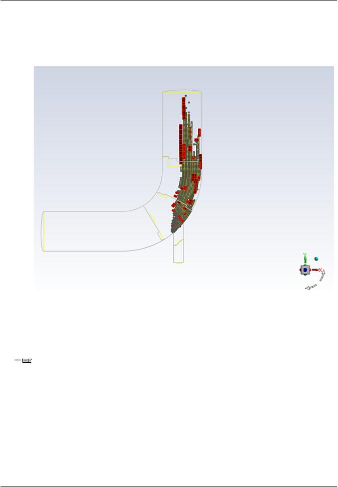
ix.Rotate the view and zoom in to get the display shown in Figure 2.13: Alternative Display of Cells Marked for Adaption (p. 85).

Figure 2.13: Alternative Display of Cells Marked for Adaption

x.After viewing the marked cells, rotate the view back and zoom out again.

xi.Click OK to close the Adaption Controls dialog box.

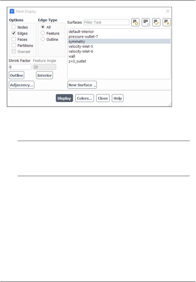
3.Display the adapted mesh (Figure 2.14: The Adapted Mesh (p. 87)).

Domain → Mesh → Display...

vk.com/club152685050Fluid Flow and Heat Transfer| vk.incom/id446425943a Mixing Elbow

a.Select All from the Edge Type list.

b.Deselect all of the highlighted items from the Surfaces selection list except for symmetry.

Tip

To deselect all surfaces, click the Deselect All Shown button () at the top of the Surfaces selection list. Then select the desired surface from the Surfaces selection list.

c. Click Display and close the Mesh Display dialog box.

4.Request an additional 90 iterations.

Solution → Run Calculation → Calculate

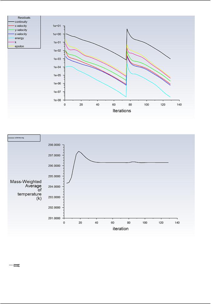
The solution will converge as shown in Figure 2.15: The Complete Residual History (p. 88) and Figure 2.16: Convergence History of Mass-Weighted Average Temperature (p. 88).

vk.com/club152685050Fluid Flow and Heat Transfer| vk.incom/id446425943a Mixing Elbow

Figure 2.15: The Complete Residual History

Figure 2.16: Convergence History of Mass-Weighted Average Temperature

5.Save the case and data files for the Coupled solver solution with an adapted mesh (elbow2.cas.gz and elbow2.dat.gz).

File → Write → Case & Data...

a.Enter elbow2.gz for Case/Data File.

b.Click OK to save the files and close the Select File dialog box.

The files elbow2.cas.gz and elbow2.dat.gz will be saved in your default folder.

6.Display the temperature distribution (using node values) on the revised mesh using the temperature contours definition that you created earlier (Figure 2.17: Filled Contours of Temperature Using the Adapted

Mesh (p. 89)).

Right-click the Results/Graphics/Contours/contour-temp tree item and select Display from the menu that opens.

Figure 2.17: Filled Contours of Temperature Using the Adapted Mesh

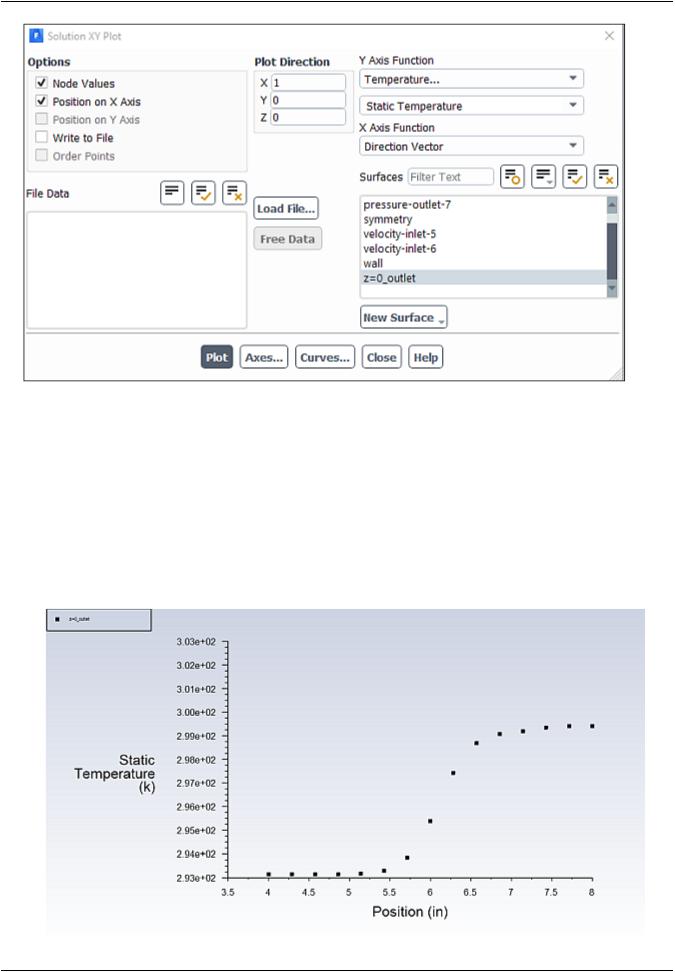
7.Display and save an XY plot of the temperature profile across the centerline of the outlet for the adapted solution (Figure 2.18: Outlet Temperature Profile for the Adapted Coupled Solver Solution (p. 90)).

Results → Plots → XY Plot → Edit...

vk.com/club152685050Fluid Flow and Heat Transfer| vk.incom/id446425943a Mixing Elbow

a.Ensure that the Write to File option is disabled in the Options group box.

b.Ensure that Temperature... and Static Temperature are selected from the Y Axis Function drop-down lists.

c.Ensure that z=0_outlet is selected from the Surfaces selection list.

d.Click Plot.

Figure 2.18: Outlet Temperature Profile for the Adapted Coupled Solver Solution

e.Enable Write to File in the Options group box.

The button that was originally labeled Plot will change to Write....

f.Click Write....

i.In the Select File dialog box, enter outlet_temp2.xy for XY File.

ii.Click OK to save the temperature data.

g.Close the Solution XY Plot dialog box.

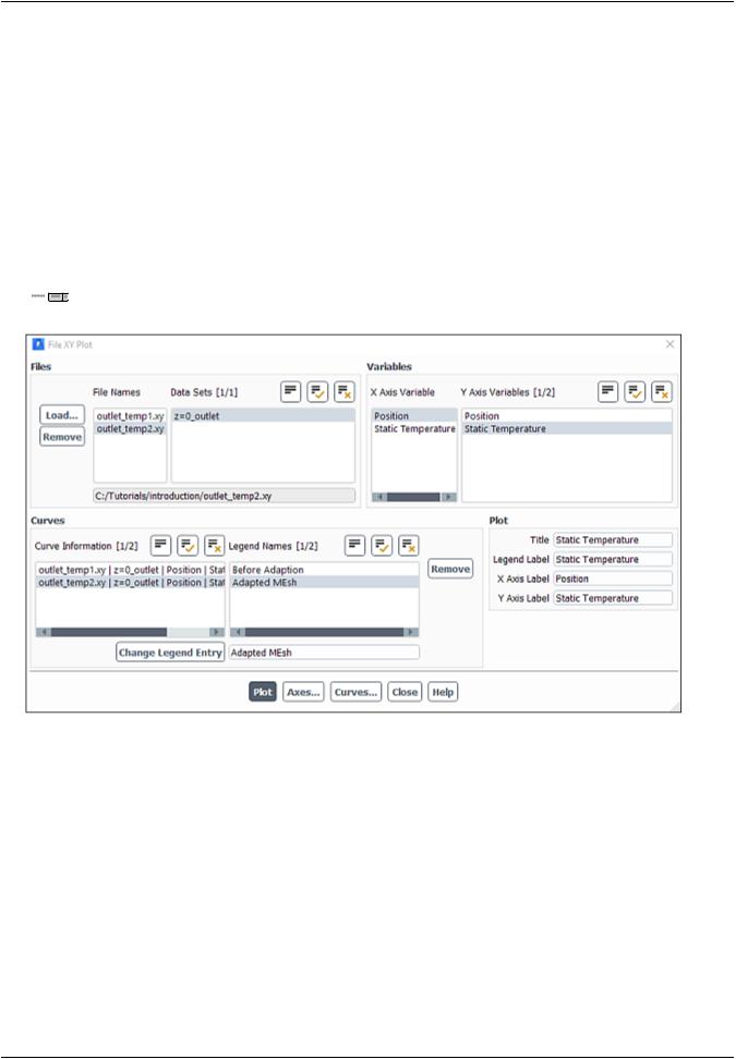
8.Display the outlet temperature profiles for both solutions on a single plot (Figure 2.19: Outlet Temperature Profiles for the Two Solutions (p. 93)).

Results → Plots → File...

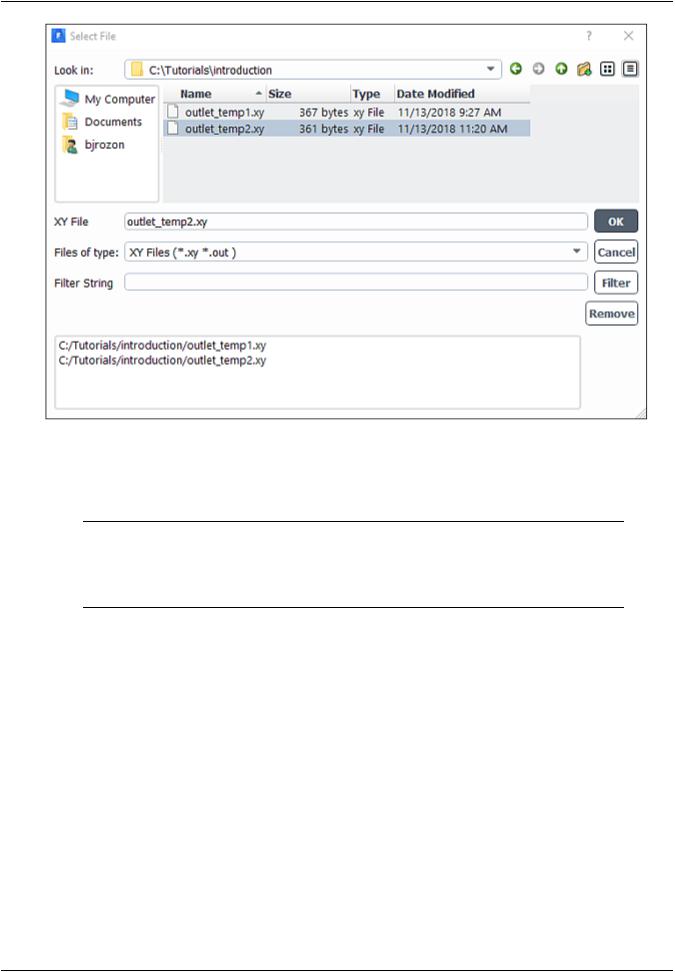
a. Click the Load... button to open the Select File dialog box.

vk.com/club152685050Fluid Flow and Heat Transfer| vk.incom/id446425943a Mixing Elbow

i.Click once on outlet_temp1.xy and outlet_temp2.xy.

Each of these files will be listed with their folder path in the bottom list to indicate that they have been selected.

Tip

If you select a file by mistake, simply click the file in the bottom list and then click Remove.

ii. Click OK to save the files and close the Select File dialog box.

b.Select the folder path ending in outlet_temp1.xy from the Curve Information selection list.

c.Enter Before Adaption in the lower-right text-entry box.

d.Click the Change Legend Entry button.

The item in the Legend Entries list for outlet_temp1.xy will be changed to Before Adaption. This legend entry will be displayed in the upper-left corner of the XY plot generated in a later step.

e.In a similar manner, change the legend entry for the folder path ending in outlet_temp2.xy to be Adapted Mesh.

f.Click Plot and close the File XY Plot dialog box.

Figure 2.19: Outlet Temperature Profiles for the Two Solutions (p. 93) shows the two temperature profiles

at the centerline of the outlet. It is apparent by comparing both the shape of the profiles and the predicted