vk.com/club152685050Using the Multiphase Models| vk.com/id446425943

19.4.5. Materials

The default properties for water defined in ANSYS Fluent are suitable for this problem. In this step, you will make sure that this material is available for selecting in future steps.

1.Add water to the list of fluid materials by copying it from the ANSYS Fluent materials database.

Setup → Materials → Fluid → air → Edit...

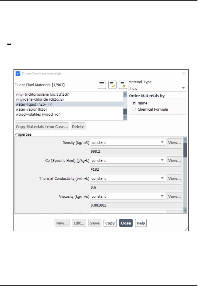
a.Click Fluent Database... in the Create/Edit Materials dialog box to open the Fluent Database Materials dialog box.

i.Select water-liquid (h2o<l>) in the Fluent Fluid Materials selection list.

Scroll down the list to find water-liquid (h2o<l>). Selecting this item will display the default properties in the dialog box.

ii.Click Copy and close the Fluent Database Materials dialog box.

The Create/Edit Materials dialog box will now display the copied properties for water-liquid.

b. Click Change/Create and close the Create/Edit Materials dialog box.

19.4.6. Phases

In the following steps you will define the liquid water and air phases that flow in the mixing tank.

1. Specify liquid water as the primary phase.

Setup → Models → Multiphase → Phases → phase-1 Edit...

a.Enter water for Name.

b.Select water-liquid from the Phase Material drop-down list.

c.Click OK to close the Primary Phase dialog box.

2.Specify air as the secondary phase.

Setup → Models → Multiphase → Phases → phase-2 Edit...

a.Enter air for Name.

b.Retain the default selection of air from the Phase Material drop-down list.

c.Enter 0.0015 m for Diameter.

The diameter of the air bubbles that are formed when the air is injected into the tank depends on the diameter of the inlet holes in the real reactor, which is 1 mm in this example.

d.Click OK to close the Secondary Phase dialog box.

3.Define the interphase interactions formulations to be used.

Setup → Models → Multiphase → Phases → Phases Interactions Edit...

a.In the Drag tab, select grace from the Drag Coefficient drop-down list.

The Grace model is suitable for liquid-gas mixtures with low gas density and bubble sizes of 1-2 mm.

Click OK to close the Grace Swarm Correction dialog box.

b.In the Surface Tension tab, select constant from the Surface Tension Coefficients drop-down list and enter 0.073.

c.Click OK to close the Phase Interaction dialog box.

19.4.7. Cell Zone Conditions

The mesh has three fluid cell zones: fluid_mrf_1-1 and fluid_mrf_2-0 are zones associated with the Rushton blade turbine and pitch blade turbine, respectively, and fluid_tank-2 represents the rest of the tank. In this section, you will use multiple reference frames to define boundary conditions for the cell zones that contain rotating components. Moving reference frames enable you to model the flow around rotating parts as steadystate with respect to the moving frames.

vk.com/club152685050Using the Multiphase Models| vk.com/id446425943

Physics → Zones → Cell Zones...

Tip

To visually confirm the location of a cell or boundary zone, you can display it by right-clicking it in the tree and selecting either Display or Add to Graphics. Conversely, if you click a cell or boundary mesh in the graphics window, the selected item will be highlighted in the tree. You can use Ctrl or Shift to select multiple zones.

1.Set up the cell zone conditions for the fluid zone associated with the Rushton blade turbine (fluid_mrf_1- 1).

Setup → Cell Zone Conditions → fluid_mrf_1-1 Edit...

a.In the Fluid dialog box, enter rbt-zone for Zone Name.

This name is more descriptive for the zone than fluid_mrf_1-1.

b.Select Frame Motion.

c.Retain the default values of (0, 0, 1) for X, Y, and Z in the Rotation-Axis Direction group box.

d.Enter 450 rpm for Speed in the Rotational Velocity group box.

e.Click OK to close the Fluid dialog box.

2.In a similar manner, set up the cell zone conditions for the fluid zone associated with the pitch blade turbine (fluid_mrf_2-0).

Setup → Cell Zone Conditions → fluid_mrf_2-0 Edit...

a.In the Fluid dialog box, enter pbt-zone for Zone Name.

b.Select Frame Motion.

c.Retain the default values of (0, 0, 1) for X, Y, and Z in the Rotation-Axis Direction group box.

d.Enter 450 rpm for Speed in the Rotational Velocity group box.

e.Click OK to close the Fluid dialog box.

3.Retain the default settings for fluid_tank-2, which is stationary in the absolute reference frame.

19.4.8. Boundary Conditions

You will now define the conditions on the boundaries of the domain. Since each wall uses the same reference frame as the cell zone within which they are located, all walls will use the default stationary wall condition.

A stationary wall condition implies that the wall is stationary with respect to the adjacent cell zone. Therefore, in the case of a rotating reference frame, a stationary wall is actually rotating with respect to the absolute reference frame.

The degassing boundary condition at the top of the fluid was created in a meshing application. At the degassing outlet, only gas phase can leave the domain. The degassing boundary condition became active after you enabled the Eulerian multiphase model in Fluent. No input is required for this type of boundary condition. For this problem, you only need to set the boundary conditions for the velocity inlet. Since this is a multiphase model, you will set the conditions that are specific to the primary and secondary phases.

1. Set the boundary conditions at the inlet (gas-inlet) for the primary phase (water).

Setup → Boundary Conditions → gas-inlet → water Edit...

Since this is a dispersed turbulent flow, only turbulence must be defined for the water phase.

a.In the Turbulence group box, select Intensity and Hydraulic Diameter as the turbulence Specification Method.

b.Enter 3% for Turbulent Intensity.

c.Enter 0.0254 m for Hydraulic Diameter.

d.Click OK to close the Velocity Inlet dialog box.

2.Set the boundary conditions at the inlet (gas-inlet) for the secondary phase (air).

Setup → Boundary Conditions → gas-inlet → air Edit...

a.Enter 0.05 m/s for Velocity Magnitude.

b.In the Multiphase tab, enter 1 for Volume Fraction.

A value of unity implies that only air enters the inlet.

c.Click OK to close the Velocity Inlet dialog box.

19.4.9. Solution

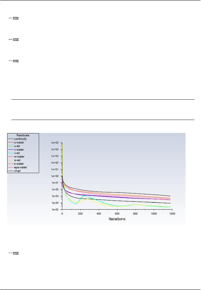
2.Ensure that the plotting of residuals is enabled during the calculation.

Solution → Reports → Residuals...

vk.com/club152685050Using the Multiphase Models| vk.com/id446425943

3.Initialize the solution.

Solution → Initialization → Initialize

4.Save the case file (mixing_tank.cas.gz).

File → Write → Case...

5.Start calculation.

Solution → Run Calculation → Advanced...

a.Enter 1500 for Number of Iterations.

b.Retain the default selection of Automatic for the Time Step Method.

c.Retain the default value of 1 for Timescale Factor.

Note

It may take significant time and computer resources to complete the problem calculation.

Figure 19.3: Residual History

6.After the solution has converged, save the case and data files (mixing_tank.cas.gz and mixing_tank.dat.gz).

File → Write → Case & Data...