vk.com/club152685050Fluid Flow and Heat Transfer| vk.incom/id446425943a Mixing Elbow

solution procedure, you should set reasonable backflow conditions to prevent convergence from being adversely affected.

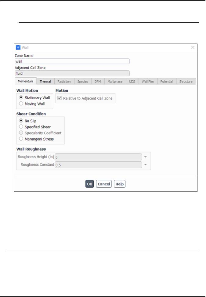
e. For the wall of the pipe (wall), retain the default value of 0 W/m2 for Heat Flux in the Thermal tab.

2.4.6. Solving

In the steps that follow, you will set up and run the calculation using the Solution ribbon tab.

Note

You can also use the task pages listed under the Solution tree branch to perform solutionrelated activities.

1.Select a solver scheme.

a. In the Solution ribbon tab, click Methods... (Solution group box).

Solution → Solution → Methods...

b. Retain the default selections.

2.Enable the plotting of residuals during the calculation.

vk.com/club152685050Fluid Flow and Heat Transfer| vk.incom/id446425943a Mixing Elbow

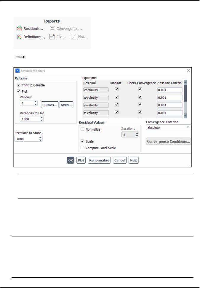
a. In the Solution ribbon tab, click Residuals... (Reports group box).

Solution → Reports → Residuals...

Note

You can also access the Residual Monitors dialog box by double-clicking the Solution/Monitors/Residual tree item.

b.Ensure that Plot is enabled in the Options group box.

c.Retain the default value of 0.001 for the Absolute Criteria of continuity.

d.Click OK to close the Residual Monitors dialog box.

Note

By default, the residuals of all of the equations solved for the physical models enabled for your case will be monitored and checked by ANSYS Fluent as a means to determine the convergence of the solution. It is a good practice to also create and plot a surface report definition that can help evaluate whether the solution is truly converged. You will do this in the next step.

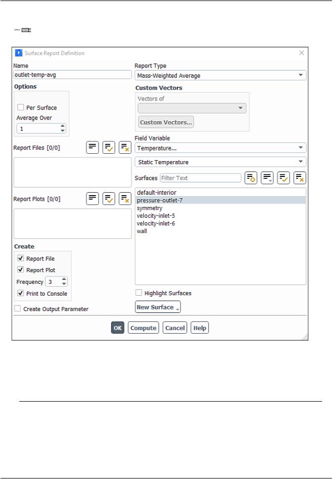
3.Create a surface report definition of average temperature at the outlet (pressure-outlet-7).

Solution → Reports → Definitions → New → Surface Report → Mass-Weighted Average...

Note

You can also access the Surface Report Definition dialog box by right-clicking Report Definitions in the tree (under Solution) and selecting New/Surface Report/MassWeighted Average... from the menu that opens.

a.Enter outlet-temp-avg for the Name of the report definition.

b.Enable Report File, Report Plot, and Print to Console in the Create group box.

During a solution run, ANSYS Fluent will write solution convergence data in a report file, plot the solution convergence history in a graphics window, and print the value of the report definition to the console.

vk.com/club152685050Fluid Flow and Heat Transfer| vk.incom/id446425943a Mixing Elbow

c.Set Frequency to 3 by clicking the up-arrow button.

This setting instructs ANSYS Fluent to update the plot of the surface report, write data to a file, and print data in the console after every 3 iterations during the solution.

d.Select Temperature... and Static Temperature from the Field Variable drop-down lists.

e.Select pressure-outlet-7 from the Surfaces selection list.

f.Click OK to save the surface report definition and close the Surface Report Definition dialog box.

The new surface report definition outlet-temp-avg will appear under the Solution/Report Definitions tree item. ANSYS Fluent also automatically creates the following items:

•outlet-temp-avg-rfile (under the Solution/Monitors/Report Files tree branch)

•outlet-temp-avg-rplot (under the Solution/Monitors/Report Plots tree branch)

4.In the tree, double-click outlet-temp-avg-rfile (under Solution/Monitors/Report Files) and examine the report file settings in the Edit Report File dialog box.

The dialog box is automatically populated with data from the outlet-temp-avg report definition.

a.Verify that outlet-temp-avg is in the Selected Report Definitions list.

If you had created multiple report definitions, the additional ones would be listed under Available Report Definitions, and you could use the Add>> and <<Remove buttons to manage which were written in this particular report definition file.

b.(optional) Edit the name and location of the resulting file as necessary using the Output File Base Name field or Browse... button.

c.Click OK to close the Edit Report File dialog box.

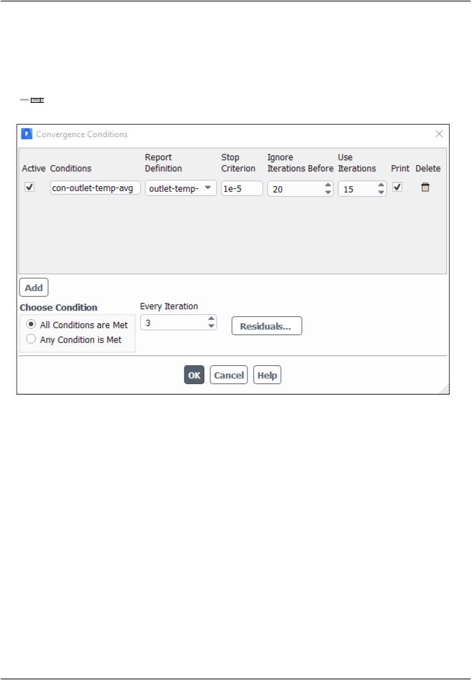
5.Create a convergence condition for outlet-temp-avg.

Solution → Reports → Convergence...

a.Click the Add button.

b.Enter con-outlet-temp-avg for Conditions.

c.Select outlet-temp-avg from the Report Definition drop-down list.

d.Enter 1e-5 for Stop Criterion.

e.Enter 20 for Ignore Iterations Before.

f.Enter 15 for Use Iterations.

g.Enable Print.

h.Set Every Iteration to 3.

i.Click OK to save the convergence condition settings and close the Convergence Conditions dialog box.

These settings will cause Fluent to consider the solution converged when the surface report definition value for each of the previous 15 iterations is within 0.001% of the current value. Convergence of the values will be checked every 3 iterations. The first 20 iterations will be ignored, allowing for any initial

vk.com/club152685050Fluid Flow and Heat Transfer| vk.incom/id446425943a Mixing Elbow

solution dynamics to settle out. Note that the value printed to the console is the deviation between the current and previous iteration values only.

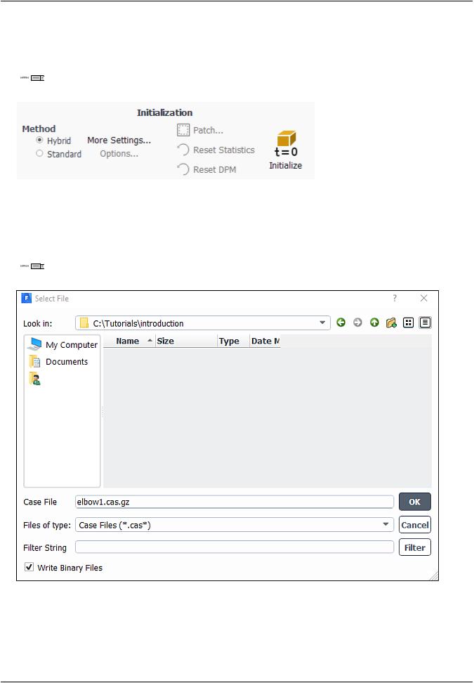
6.Initialize the flow field using the Initialization group box of the Solution ribbon tab.

Solution → Initialization

a.Retain the default selection of Hybrid from the Method list.

b.Click Initialize.

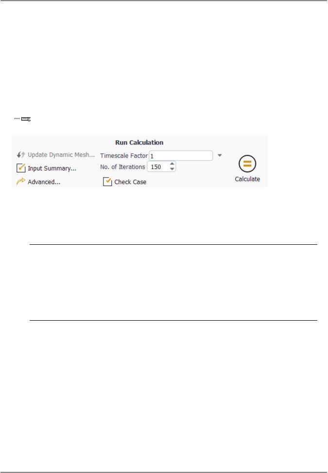
7.Save the case file (elbow1.cas.gz).

File → Write → Case...

a.(optional) Indicate the folder in which you would like the file to be saved.

By default, the file will be saved in the folder from which you read in elbow.msh (that is, the introduction folder). You can indicate a different folder by browsing to it or by creating a new folder.

b. Enter elbow1.cas.gz for Case File.

Adding the extension .gz to the end of the file name extension instructs ANSYS Fluent to save the file in a compressed format. You do not have to include .cas in the extension (for example, if you enter elbow1.gz, ANSYS Fluent will automatically save the file as elbow1.cas.gz).

The .gz extension can also be used to save data files in a compressed format.

c.Ensure that the default Write Binary Files option is enabled, so that a binary file will be written.

d.Click OK to save the case file and close the Select File dialog box.

8.Start the calculation by requesting 150 iterations in the Solution ribbon tab (Run Calculation group box).

Solution → Run Calculation

a.Enter 150 for No. of Iterations.

b.Click Calculate.

Note

By starting the calculation, you are also starting to save the surface report data at the rate specified in the Surface Report Definition dialog box. If a file already exists in your working directory with the name you specified in the Edit Report File dialog box, then a Question dialog box will open, asking if you would like to append the new data to the existing file. Click No in the Question dialog box, and then click OK in the Warning dialog box that follows to overwrite the existing file.

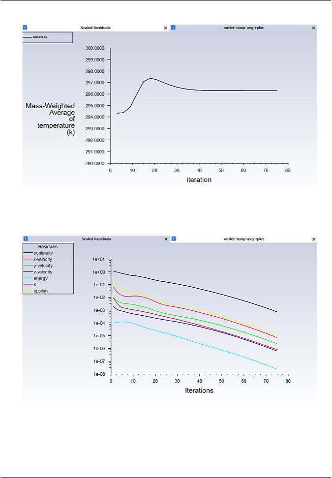
As the calculation progresses, the surface report history will be plotted in the outlet-temp-avg- rplot tab in the graphics window (Figure 2.3: Convergence History of the Mass-Weighted Average Temperature (p. 66)).

vk.com/club152685050Fluid Flow and Heat Transfer| vk.incom/id446425943a Mixing Elbow

Figure 2.3: Convergence History of the Mass-Weighted Average Temperature

Similarly, the residuals history will be plotted in the Scaled Residuals tab in the graphics window (Figure 2.4: Residuals (p. 66)).

Figure 2.4: Residuals

Note

You can monitor the two convergence plots simultaneously by right-clicking a tab in the graphics window and selecting SubWindow View from the menu that opens. To

return to a tabbed graphics window view, right-click a graphics window title area and select Tabbed View.

Since the residual values vary slightly by platform, the plot that appears on your screen may not be exactly the same as the one shown here.

The solution will be stopped by ANSYS Fluent when any of the following occur:

•the surface report definition converges to within the tolerance specified in the Convergence Conditions dialog box

•the residual monitors converge to within the tolerances specified in the Residual Monitors dialog box

•the number of iterations you requested in the Run Calculation task page has been reached

In this case, the solution is stopped when the convergence criterion on outlet temperature is satisfied. The exact number of iterations for convergence will vary, depending on the platform being used. An Information dialog box will open to alert you that the calculation is complete. Click OK in the Information dialog box to proceed.

9.Examine the plots for convergence (Figure 2.3: Convergence History of the Mass-Weighted Average Temperature (p. 66) and Figure 2.4: Residuals (p. 66)).

Note

There are no universal metrics for judging convergence. Residual definitions that are useful for one class of problem are sometimes misleading for other classes of problems. Therefore it is a good idea to judge convergence not only by examining residual levels, but also by monitoring relevant integrated quantities and checking for mass and energy balances.

There are three indicators that convergence has been reached:

•The residuals have decreased to a sufficient degree.

The solution has converged when the Convergence Criterion for each variable has been reached. The default criterion is that each residual will be reduced to a value of less than 10–3, except the energy residual, for which the default criterion is 10–6.

•The solution no longer changes with more iterations.

Sometimes the residuals may not fall below the convergence criterion set in the case setup. However, monitoring the representative flow variables through iterations may show that the residuals have stagnated and do not change with further iterations. This could also be considered as convergence.

•The overall mass, momentum, energy, and scalar balances are obtained.

You can examine the overall mass, momentum, energy and scalar balances in the Flux Reports dialog box. The net imbalance should be less than 0.2 % of the net flux through the domain when the solution has converged. In the next step you will check to see

if the mass balance indicates convergence.