2.2 Topological matrices

For an analytical description of electric circuit graphs and their storage in computer memory in a digital form it is more convenient to represent graphs in the form of topological matrices. There are incidence matrices (node matrices), loop matrices and graph section matrices.

2.2.1 Incidence matrices

It is said that if the node is the end of the branch then they are incident. Information contained in a directed graph can be fully represented by a matrix called incidence matrix (node matrix).

The matrix is called the incidence matrix which corresponds to the directed graph with “ ” nodes and “ ” branches

(2.1)

where is the element of the matrix;

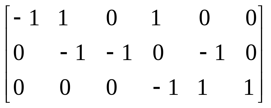
=1 if the branch is incident to the node and directed from the node; =-1 if the branch is incident to the node and directed to the node; =0 if the branch is not incident to the node . For instance, we will obtain the matrix (2.2) for the directed graph according to Fig. 2.3,c. It’s clear from the matrix that the number of non – zero elements in each line of the matrix is equal to the number of branches incident to the corresponding node. Each column contains only

branches

= (2.2)

incident branches

two non – zero elements: “+1” and “-1” because each branch is incident to two nodes and directed from one of them to the other. The sum of all elements of each column and, consequently, the sum of all matrix lines is equal to zero, i.e. the matrix lines are linearly dependent. Therefore, it’s possible to exclude any line of the matrix without any information loss. So, when the 4-th line is excluded in (2.2) we get:

= (2.3)

Matrix is called the reduced incidence matrix.

2.2.2 The loop matrix

Topological matrixes can be compiled for circuit loops too.

= (2.4)

where, are elements of the matrix . =1 if the branch is incident to the loop and coincides with the direction of loop path-tracing; =-1 if the branch is incident to the loop and opposite to the direction of loop path tracing; =0 if the branch is not incident to the loop . The loop matrix corresponding to the directed graph with “ ” loops and “ ” branches, is the name for the matrix . For instance, for the directed graph in Fig. 2.3,c we will get the matrix (2.5) when loop path-tracing is clockwise. Here, the branch of the current source is not used in the matrix because such a branch does not form a separate loop as mentioned above.

It’s obvious that the parts of loops not used in the matrix (2.5) are linearly dependent. A loop, that includes at least one branch not being part of any other loops, is linearly independent.

branches

=

loops

For the planar circuits it’s easy to define the number of independent loops if we take these loops as meshes of the graph grid or “windows”. So for the graph in Fig.2.3,c the loops will be the following: Then we get the submatrix from the matrix .

= (2.6)

The matrix is called the matrix of main loops.

For nonplanar circuits, it is difficult to define the number of dependent loops from the number of “windows” in the graph. In this case, the T graph tree is used. A loop is formed by the connection of any chord to a tree. This loop is called the main loop. The direction of main loop path-tracing is taken as the chord direction. Thus, the number of main loops is equal to the number of chords of the selected graph tree. It is evident that it is equal to . So, main loops for the tree in Fig. 2.3,b are formed by the chords: chord loop chord loop chord loop Having arranged the edges in the lower columns, we get the matrix of main loops for the graph with the tree in Fig. 2.3,b

Tree chords

= (2.7)

As seen from (2.7), any matrix can be divided in the following way:

= (2.8)

where matrix corresponds to the edges

edges

= (2.9)

chords

Matrix 1 is a unit matrix and corresponds to the chords

edges

1= (2.10)

chords

So, because the unit matrix is present in the matrix , we can say that the lines of the matrix are linearly independent.