Supersymmetry. Theory, Experiment, and Cosmology

370 A review of the Standard Model and of various notions of quantum field theory

Comparison with the abelian case is more transparent in the case of infinitesimal transformations:

In order to expand (A.43) we need the commutator of two generators. In the general case, we have

where the Cabc are the structure constants of the group G. Comparison with (A.26) shows that, in the case of SU (2), Cabc = abc. One then easily obtains from expanding (A.43) to linear order in αa,

The last term is similar to the abelian case in (A.31). The second term is specific to the nonabelian situation: it involves the nonvanishing structure constants Cabc of the nonabelian gauge group. Introducing the generators T a in the adjoint representation ((T a)bc = −iCabc), one may write the infinitesimal transformation (A.46) as

It remains to write a dynamics for the vector fields, and thus to define a field strength. By analogy with the abelian case, we may consider ∂µAν − ∂ν Aµ. Using (see exercise 2)

From the form of the first term on the right-hand side, it is clearly hopeless to expect a gauge invariant field strength as in the abelian case. We may at best expect that Fµν transforms as U Fµν U −1: a covariant field strength. Indeed, because

Symmetries 371

We could have obtained directly the field strength from the commutation of two covariant derivatives (as in the abelian case):

We also note that T r F µν Fµν is invariant. Since Fµν is a N × N matrix, we may write it Fµν = Fµνa ta where, from (A.45) and (A.49)

as in (A.25), we have 12 Tr(F µν Fµν ) = 14 F aµν Fµνa . As in the abelian case, the fermion– gauge field coupling is of the form

One important di erence between abelian and nonabelian gauge theories is the notion of charge or quantum number. In (A.29) and (A.32), we have included a real number q whose value is not fixed by the symmetry. If we try to introduce such a number in the nonabelian case and replace (A.37) and (A.38), respectively, by

then it is easy to show that DµΨ is covariant under an infinitesimal transformation only if X = 0 or 1. This shows that, in a nonabelian gauge theory, charges (i.e. quantum numbers) can only take quantized values fixed by group theory (i.e. matrix elements of generators ta). This will be one of the motivations for embedding the quantum electrodynamics U (1) symmetry into a nonabelian grand unified gauge symmetry group.

372 A review of the Standard Model and of various notions of quantum field theory

A.2 Spontaneous breaking of symmetry

A.2.1 Example of a global symmetry

We start with the simplest example of a global abelian symmetry and consider a complex scalar field φ(x) with a Lagrangian density

This has a global phase invariance φ(x) → φ (x) = e−iθφ(x) ; and the associated conserved Noether current is Jµ = −iφ∂µφ†+iφ†∂µφ. Requirement of renormalizability imposes to limit the interaction potential V to quartic terms:

where λ > 0 to avoid instability at large values of the field. The corresponding equation of motion reads:

If a > 0, we may write a ≡ m2 and the equation of motion

where j(φ) ≡ −λφ(φ†φ) describes the self-interaction of the field φ. It is then possible to quantize the theory: first quantize the free field theory corresponding to vanishing self-interaction (the field obeys the Klein–Gordon equation ( + m2)φ = 0) and then use perturbation theory in λ.

We are interested in the vacuum structure of the theory, i.e. in identifying its ground state. Using Noether formalism, one may compute the energy of the system

P0 = d3x H(x)

where π (resp. π†) is the canonical conjugate momentum of φ(x) (resp. φ†(x)) as in (A.16). This gives in the present case:

Since the first two terms are positive definite, minimization of the energy density is obtained by setting them to zero, i.e. by taking a constant value for the field φ, and by minimizing the potential energy. In other words, we minimize the energy density by choosing a constant value φ0 which corresponds to the minimum of V . If a ≥ 0, the minimum is at φ = 0 (see Fig. A.1) i.e. for vanishing field. We are familiar with this situation: for example, the electromagnetic energy density 81π (E2 + B2) is minimized for E = B = 0. In this latter case, a nonvanishing electric or magnetic field in the vacuum (i.e. the ground state) would obviously break the isotropy of space. There is no such risk with a scalar field.

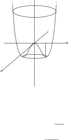
374 A review of the Standard Model and of various notions of quantum field theory

V (φ)

Im φ

Fig. A.2

form linear combinations of ground states which are invariant under the symmetry. This is not possible in the case of quantum field theory because of the infinite number of degrees of freedom (infinite volume): the mixed Hamiltonian matrix elements between two di erent ground states vanish.

Now, following our remark above, let us return to our example and express the scalar field around its ground state value, say eiθ0 "m2/λ. We write

We conclude that the field ϕ1 has mass squared 2m2 (beware of the normalization of the kinetic term 12 ∂µϕ1∂µϕ1) whereas ϕ2 is massless. Thus the mass spectrum does not reflect the symmetry: even though ϕ1 and ϕ2 are interchanged in the symmetry transformation, they are not degenerate in mass. This is a consequence of the spontaneous breaking of the symmetry. Moreover, the fact that ϕ2 is massless is not a coincidence. Indeed, it is a general theorem due to [198] that to every continuous global symmetry spontaneously broken, there corresponds a massless particle. In the case of internal symmetries such as considered here, it is a boson called the Goldstone boson.

376A review of the Standard Model and of various notions of quantum field theory

[83]has shown that a symmetry of the vacuum is a symmetry of the Hamiltonian1. But the converse is not true. If [Q, H] = 0 or ∂µjµ = 0, then one may distinguish two cases:

(a) Wigner realization Q|0 = 0

This has well-known properties. Two states which transform into one another under the symmetry are degenerate in energy. Indeed, if φ = U †φU , then

0|φ †Hφ |0 = 0|U †φ†U HU †φ U |0 = 0|φ†Hφ|0 ,

using both (A.73) and (A.74).

Also, Green’s functions (i.e. the vacuum values of chronological products of fields0|T φ(x1) · · · φ(xn)|0 ) are invariant under the symmetry: this leads to Ward identities which translate the symmetry at the level of Green’s functions. Indeed, under an infinitesimal transformation, using (A.17) (which is derived from (A.13) or (A.71)), we have, for x01 > x02 > · · · > x0n,

δ 0|T φ(x1) · · · φ(xn)|0 = 0|δφ(x1)φ(x2) · · · φ(xn)|0

+ 0|φ(x1)δφ(x2) · · · φ(xn)|0 + · · ·

=iδα 0|(Qφ(x1) − φ(x1)Q)φ(x2) · · · φ(xn)|0

+iδα 0|φ(x1)(Qφ(x2) − φ(x2)Q) · · · φ(xn)|0 + · · ·

=0.

(b)Goldstone realization Q|0 = 0

Two states which are exchanged under the symmetry are not necessarily degenerate. Hence the symmetry is not manifest in the energy (mass) spectrum. We have seen an explicit example of this in the previous Section. The symmetry is said2 to be spontaneously broken.

According to case (a), it su ces to prove that at least one Green’s function is not invariant: δ 0|T φ(x1) · · · φ(xn)|0 = 0. In most cases, it is the one-field Green’s function 0|φ(x)|0 which is not invariant: in other words, the vacuum expectation value of a field is not invariant. This was precisely the case of the explicit example presented in the previous Section. We now prove Goldstone’s theorem in this case.

Defining

we see that η = 0 because the symmetry is not an invariance of the vacuum (expressed as 0 = 0|δφ(x)|0 = i 0[Q, φ(x)]|0 using (A.17)) whereas dη/dt = 0 because the symmetry is an invariance of the Hamiltonian (i.e. the charge is a constant of motion: dQ/dt = i[H, Q] = 0).

d3xj0(t, x)|0 = 0. If |n is a state of vanishing 3-momentum, one may apply the bra n| to the previous relation. Thus, n| d3xe−ik·xj0(t, x)|0 = 0 and n|j0(x)|0 = 0 from which follows n|∂µjµ(x)|0 = 0. Lorentz invariance implies that this is true for any state |n and thus ∂µjµ(x)|0 = 0 from which (A.72) follows.

2Somewhat improperly since the symmetry remains an invariance of the Hamiltonian.

Spontaneous breaking of symmetry 377

We introduce a complete basis of eigenstates |n of energy (H|n = En|n ) and

3-momentum (P|n = pn|n ). The zero of energy is taken at the ground state: H|0 =

#

E0|0 = 0, P|0 = p0|0 = 0. Then using the closure relation n |n n| = 1l, and translation operators:

J0(t, x) = e−ip·xeiHtJ0(0)e−iHteip·x,

we may write η as:

n &

=d3x e−iEnteipn·x 0|J0|n n|φ(0)|0

−eiEnte−ipn·x 0|φ(0)|n n|J0)|0

&

=(2π)3δ3(pn) e−iEnt 0|J0|n n|φ(0)|0

For this to be identically vanishing, whereas η = 0, there must be a state |n0 such that En0 δ3(pn0 ) = 0 (i.e. the state |n0 is a massless excitation of the system) and

This massless excitation is the Goldstone boson.

A.2.3 General discussion in the case of global symmetries

We now consider the general case of a group G of continuous global transformations. The scalar fields are taken to be real and transform under G as:

where the ta are the generators of the group, in a n-dimensional representation3. Infinitesimally

where m = 1, . . . , n.

3The ta are taken to be hermitian, ta† = ta. Since φ is real, (ita) = ita. Hence ta = −ta and taT = −ta: the generators are antisymmetric.