Supersymmetry. Theory, Experiment, and Cosmology

The hot Big Bang scenario 469

D.3.3 Relics

In this book, we pay specific attention to the evolution of the abundance of stable or quasistable massive particles. They may provide good candidates for dark matter (see Chapter 5) or alternatively could become too abundant at present times to be consistent with observations (see Chapter 11). We have noted that the number densities of massive particles in thermal equilibrium become exponentially small for temperatures smaller than their mass. This is, however, under the assumption of thermal equilibrium. Because we are in an expanding Universe, particles may drop out of thermal equilibrium and their abundance be frozen at the corresponding temperature.

Let us consider the evolution of a given stable particle species of mass mX . There are two competing e ects which modify the abundance of this species: annihilation and expansion of the Universe. Indeed, the faster is the dilution associated with the expansion, the least e ective is the annihilation because the particles recede from one another. This is illustrated by the following equation which gives the evolution with time of the particle number density nX :

as given in (D.57). The friction term 3HnX in (D.70) represents the e ect of the expansion of the Universe: in the absence of the annihilation process, the number of

Because of annihilation, the evolution equation has two regimes:

•As long as the expansion rate H is smaller than the annihilation rate ΓX ≡ nX σannv , one may solve (D.70) disregarding the expansion: nX /T 3 n(eq)X /T 3 exp (−mX /kT ). Obviously, as time goes on, T decreases, the energy density nX decreases and so does the annihilation rate.

•Once the expansion rate H becomes larger than the annihilation rate ΓX , there is freezing of the number of particles in a covolume and n/T 3 becomes constant. This occurs at a freezing temperature Tf such that

The explicit form of nX (Tf ) depends crucially on whether the species is still relativistic at the time of freezing. We start with the case of cold relics, which are nonrelativistic at the time of freezing. Let us define xf ≡ mX /(kTf ). Using (D.60), with gX number of degrees of freedom of the X particle, and (D.62), one obtains

The hot Big Bang scenario 471

D.3.4 Cosmic microwave background

Before discussing the spectrum of CMB fluctuations, we introduce the important notion of a particle horizon in cosmology.

Because of the speed of light, a photon which is emitted at the Big Bang (t = 0) will have travelled a finite distance at time t. The proper distance (D.20) measured at time t is simply given as in (D.41) by the integral:

where, in the second line, we have used (D.46). This is the maximal distance that a photon (or any particle) could have travelled at time t since the Big Bang . In other words, it is possible to receive signals at a time t only from comoving particles within a sphere of radius dh(t). This distance is known as the particle horizon at time t.

A quantity of relevance for our discussion of CMB fluctuations is the horizon at the time of the recombination i.e. zrec 1100. We note that the integral on the second line of (D.79) is dominated by the lowest values of z: z zrec where the Universe is still matter dominated. Hence

We note that this is simply twice the Hubble radius at recombination H−1(zrec ), as can be checked from (D.45):

This radius is seen from an observer at present time under an angle

where the angular distance has been defined in (D.52). We can compute analytically this angular distance under the assumption that the Universe is matter dominated (see Exercise 4). Using (D.133), we have

Thus, since, in our approximation, the total energy density ΩT is given by ΩM ,

We have written in the latter equation ΩT instead of ΩM because numerical computations show that, in case where ΩΛ is nonnegligible, the angle depends on ΩM +ΩΛ= ΩT .

The hot Big Bang scenario 473

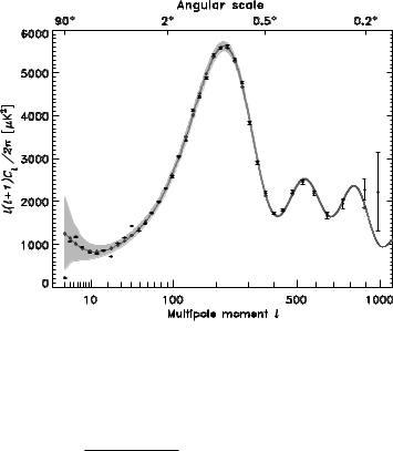
Fig. D.4 This figure compares the best-fit power law ΛCDM model to the temperature angular power spectrum observed by WMAP [225].

averaged over all n1 and n2 satisfying the condition n1 · n2 = cos θ, we have indeed

We may decompose C(θ) over Legendre polynomials:

The monopole (l = 0) related to the overall temperature T0, and the dipole (l = 1) due to the Solar system peculiar velocity bring no information on the primordial fluctuations. A given coe cient Cl characterizes the contribution of the multipole component l to the correlation function. If θ 1, the main contribution to Cl corresponds to an angular scale8 θ π/l 200◦/l. The previous discussion (see (D.84) and (D.86)) implies that we expect the first acoustic peak at a value l 200Ω−T 1/2.

The power spectrum obtained by the WMAP experiment is shown in Fig. D.4. One finds the first acoustic peak at l 200, which constrains the ΛCDM model used to perform the fit to ΩT = ΩM + ΩΛ 1. Many other constraints may be inferred from a detailed study of the power spectrum.

8The Cl are related to the coe cients alm in the expansion of ∆T /T in terms of the spherical harmonic Ylm: Cl = |alm|2 m. The relation between the value of l and the angle comes from the observation that Ylm has (l − m) zeros for −1 < cos θ < 1 and Re(Ylm) m zeros for 0 < φ < 2π.

474 An introduction to cosmology

D.3.5 Baryogenesis

It is obvious to note that the observed Universe contains much more matter than antimatter. This can be expressed in a more quantitative way. The success of the standard cosmological model predictions regarding the abundances of light elements (D, 3He, 4He and 7Li), rests on the following hypothesis on the ratio of baryon density to photon density [142]:

We have seen earlier that the present value for nγ is 411 cm−3. Since no significant amount of antimatter has been detected in our Universe, we have

We note that the photon is its own antiparticle, and thus this ratio is a measure of the unbalance between matter and antimatter. The precision on ηB has recently been improved by CMB experiments. The WMAP collaboration has measured it to be [141]:

ηB = 6.1+0.3 (D.92)

−0.2

A.D. [326] has listed the conditions necessary to dynamically generate a matter– antimatter asymmetry in an expanding Universe:

•baryon number violation;

•C and CP violation;

•deviation from thermal equilibrium.

The Standard Model fulfills in principle all these requirements. Indeed there are electroweak field configurations (sphalerons) [266] which violate B and L because the corresponding currents are anomalous in the presence of background W boson fields. The presence of sphalerons leads to e ective interactions involving left-handed fields

which violate B and L by three units each (and preserve B − L). This has no e ect at zero temperature because of the small electroweak coupling but B and L-violating processes come into thermal equilibrium as one reaches the electroweak phase transition. Between the corresponding temperature ( 100 GeV) and 1012 GeV, the processes (D.93) tend to wash out any nonzero value of B + L, except if there exists a nonvanishing B − L asymmetry.

The last of the Sakharov conditions requires a first order phase transition. As the Universe undergoes this phase transition, bubbles of the true vacuum nucleate. Particles in the high temperature plasma are partially reflected when they encounter the bubble walls; these interactions can be CP violating. To avoid the washout of the baryons thus created inside the bubble, the mass of the sphaleron (given by the height of the barrier between two true vacua) must be large compared to the temperature.

476 An introduction to cosmology

in grand unified theories. In this case their mass is of order MU /g2 where g is the value of the coupling at grand unification. Because we are dealing with stable particles with a superheavy mass, there is a danger to overclose the Universe, i.e. to have an energy density much larger than the critical density.

Indeed, if we assume the presence of at least one monopole per horizon at the time tU of their formation, the number nM of monopoles satisfies

where we have used the fact that in a radiation-dominated Universe ρ a−4 T 4. For nM near the lower bound, monopoles are too scarce to annihilate among themselves. Realistic values of the parameters in (D.97) lead to a monopole energy density which is orders of magnitude larger than the critical density. We thus need some mechanism to dilute the relic density of monopoles.

Inflation provides a remarkably simple solution to these problems: it consists in a period of the evolution of the Universe where the expansion is exponential. Indeed, if the energy density of the Universe is dominated by the vacuum energy ρvac, then (D.27) reads

is in fact observed whenever the magnitude of the Hubble parameter changes slowly

Such a space was first proposed by [104,105] with very di erent motivations and is thus called de Sitter space (described in Equations (6.40) and (6.41) of Chapter 6)9.

An important property of de Sitter space is the fact that the particle horizon size is exponentially increasing in time. Indeed, we have for the horizon size, following (D.79),

Obviously a period of inflation will ease the horizon problem. It follows from the previous equation that a period of inflation extending from ti to tf = ti+∆t contributes to the horizon size a value ceHvac∆t/Hvac, which can be very large.

9It turns out that the three choices in (D.99) correspond to the same choice as can be shown by a redefinition of the spacetime coordinates (see Chapter 7 of [275]). In what follows we will take the flat k = 0 formulation when we discuss pure de Sitter space. This is obviously no longer true when one adds matter to de Sitter space.