

Supersymmetry. Theory, Experiment, and Cosmology
.pdfThe general string picture 259
The open string
There are two possible boundary conditions for an open string
|
|
|
|
|
|
Dirichlet |
XM = constant |
|
|
|
|
(10.9) |
|||||||||||
|
|
|
|
|
|
Neumann |
|
∂XM |
|
= 0. |
|
|
|
|
|
|
|
(10.10) |
|||||
|
|
|
|
|
|
|
∂σ |
|
|
|
|
|
|
|
|||||||||
|
|
|
|
|
|
|
|
|
|
|
|
|
|
|
|
|
|
|
|
||||
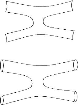
For the time being we choose the latter, which reads ∂σ XM (τ, 0) |
= 0 = |
||||||||||||||||||||||
∂σXM (τ, π) for the string of Fig. 10.2. The solution of (10.3) reads: |
|
||||||||||||||||||||||
|
|
|
|
|
|
|
|
|
|
|
|
|
|
|
|
|
|
|
|
|
|
|
|
|
M |
(z, z¯) = x |
M |
− i |
α |
M |
ln(zz¯) + i |
α |
1 |
|
M |
|
z− |
n |
+ z¯−n . |
(10.11) |
|||||||
X |
|
|
|
p |
|
|
|
|
|
|
αn |
|
|
||||||||||
|
|
2 |
|
2 |
|
n=0 n |
|
|
|||||||||||||||
The spectrum is again obtained in the light-cone formalism from a formula similar to (10.8): α M 2 = N − a. The lowest-lying states are:
•α M 2 = −a, the ground state |0 which is a tachyon;
•α M 2 = (1 − a), a set of D − 2 fields α−I 1|0 which form a vector representation of the transverse group SO(D − 2).
Again, when a = 1, i.e. D = 26, everything falls into place and the latter field is a massless vector field, with D − 2 transverse degrees of freedom. Generalizing the case of the color string, one may add nondynamical degrees of freedom (called Chan–Paton degrees of freedom) at both ends of the open string and describe them with indices i and j which run from 1 to N . There are then N 2 states at each mass level (tachyon, vector, etc.). One may go to a di erent basis (corresponding to the meson states in the case of the color string) by using the matrices λaij , a = 0, . . . , N 2 − 1:
|k; a = |
|
|
λija |k; ij . |
(10.12) |
ij
The string diagram of Fig. 10.4 represents the tree-level interaction of two open strings. The corresponding amplitude then includes a Chan–Paton factor
N |
|
|
|
|
|
|
|
λb |
λc |
λd |
(10.13) |
||
λa |
= Tr λaλbλcλd |
. |
||||
ij |
jk |
kl |
li |
|
|
|
i,j,k,l=1
It is invariant under the U (N ) transformations: λ → U λU −1. Since the corresponding N 2 massless vector fields transform as the adjoint representation of this U (N ) symmetry, this global world-sheet symmetry appears as a local gauge symmetry in spacetime.
260 An overview of string theory and string models
– |
j |
|
j |
||
a |
b |
|
i |
– |
|
k |
||
– |
k |
|
|
||
i |
c |
|
d |
||
– |
||
|
||
l |
l |
|
|
Fig. 10.4
Fig. 10.5
In the string context, the graviton exchange diagram of Fig. 10.1 is now represented by the string diagram of Fig. 10.5 which may be thought as representing the corresponding world-sheet (in as much as the Feynman diagram of Fig. 10.1 represents world-lines): from left to right two closed strings join to make a single closed string and then disjoin and get apart. Conformal invariance tells us that this surface can be deformed at will; the corresponding amplitude is not modified, as in the original Veneziano amplitude. One may then understand qualitatively how string theory avoids the small distance (ultraviolet) infinities: small distance singularities are smeared out by the process which turns Feynman diagrams for point particles into surface diagrams for extended one-dimensional objects. Indeed, string theory proves to be ultraviolet finite.
The spectrum of string oscillation modes is very rich. One may wonder how one can ever get oscillation modes which are spacetime fermions. The solution is to introduce internal (two-dimensional) “fermionic”3 degrees of freedom on the world-sheet4. Depending on their (even or odd) boundary conditions along the strings, the corresponding oscillation modes are spacetime bosons or fermions [317]. It is then possible
3In two dimensions, the distinction between fermions and bosons is artificial. In fact, one can “bosonize” the fermion fields.
4The theory on the world-sheet then has two-dimensional supersymmetry: this was in fact the first supersymmetric theory ever written. It prompted searches for a four-dimensional supersymmetric theory.

The general string picture 261
to write a string theory which has spacetime supersymmetry [194], i.e. a superstring theory.
Superstring theories are favored because they cure one problem of nonsupersymmetric theories: the requirement of supersymmetry projects out a tachyon field (i.e. a field of negative mass squared). The tachyon present in nonsupersymmetric string theories is presumably a sign of an instability of the theory.
Superstrings
|
|
|
|
|
|
|
|
M |
|
|
|
|
|
|
|
|
Let us introduce D two-dimensional fermions ψM = |
ψ−M |
, M |
= 0, . . . , |
|||||||||||||
|
|
|
|
|
|
|
ψ+ |
|
|
|
1). Their |
|||||
D |
− |
1, on the world-sheet ( refers to the two-dimensional chirality |
|
|
||||||||||||
|
± |
M |
= ψ |
M |
(τ + σ) and ψ |
M |
|
±M |
(τ |
|
σ). |
|||||
equation of motion imposes that ψ+ |
+ |
− |
= ψ |
− |
|
− |
||||||||||
|
|
M |
|
|
|
|
|
|
||||||||
We consider first the case of a closed string. A fermion ψ± |
may have periodic |
|||||||||||||||
boundary conditions |
|
|
|
|
|
|
|
|
|
|
|
|
|
|
||
|
|
ψM (τ, σ + π) = ψM (τ, σ). |
|
|
|
|
|
|
|
(10.14) |
||||||
|
|
± |
|
|
± |
|
|
|
|
|
|
|
|
|
|
|
It is then said to be in the [317] sector (R) and its expansion involves integer modes
ψM (τ, σ) = √ |
|
|
dM e−2in(τ ±σ). |
(10.15) |
2α |
||||
± |
|
n Z |
n |
|
|
|
|
||
A fermion with antiperiodic boundary conditions |
|
|||
ψ±M (τ, σ + π) = −ψ±M (τ, σ) |
(10.16) |
|||
is said to be in the [294] sector (NS) and has a half-integer mode expansion
ψM (τ, σ) = √ |
|
r |
|
2α |
bM e−2ir(τ ±σ). |
(10.17) |
|
± |
|
r |
|
|
|
Z+1/2 |
|
Standard quantization yields the following anticommutation relations:
{dmM , dnN } = −ηM N δm+n,0, |
(10.18) |
{brM , bsN } = −ηM N δr+s,0. |
(10.19) |
Since leftand right-moving modes are independent in the closed string, one may choose for each either boundary conditions. We thus have four possible sectors for the closed string: (R,R), (R,NS),(NS,R) and (NS,NS). In the case of an open string, the necessary boundary conditions are simply ψ+M (τ, π) = ±ψ−M (τ, π). Then fields in the Ramond sector (+ sign) have the following expansion:
|
1 |
√ |
|
|
|
ψM (τ, σ) = |
2α |
dM e−in(τ ±σ). |
(10.20) |
||
± |
√2 |
n |
|
||
|
|
|
|
n Z |
|

262 An overview of string theory and string models
Fields in the Neveu–Schwarz sector (− sign) have the expansion
|
1 |
√ |
|
r |
|
||
ψM (τ, σ) = |
2α |
bM e−ir(τ ±σ). |
(10.21) |
||||
|
|
||||||
± |
√2 |
r |
|
||||
|
|
|
|
|
Z+1/2 |
|
|
We have, in the open string case, only the sectors (R, R) and (NS, NS). The mass spectrum of the theory is then given bya
α M 2 = N |
− |
a, |
(10.22) |
|
where (we work in the light-cone formalism and I = 1, . . . , D − 2)
|
# |
∞ |
: αI |
αI : + |
# |
∞ |
n : dI dI : |
(R) |
|
|
N = |
n=1 |
−n |
n |
|
n=1 |
−n n |
|
(10.23) |
||
|
|
∞ |
I |
I |
: + |
|
∞ |
I I |
(NS). |
|
|
#n=1 |
: α−n |
αn |
#r=1/2 r : b−rbr : |
|
|||||
The zero-point energy is aR = 0 in the R sector and aNS = (D − 2)/16 in the NS sector.
The Ramond ground state |0 R is therefore massless. It is not unique: since dI0 does not appear in (10.23), [dI0, α M 2] = 0 and dI0|0 is also a ground state. In fact, since from (10.18) the dI0 satisfy a Cli ord algebra
d0I , d0J = δIJ , |
(10.24) |
they play the rˆole of gamma matrices in the D − 2 transverse space: their dimension is 2(D−2)/2 and they act as spinor representations of SO(D − 2). Thus, we see that the Ramond vacuum is in a (massless) spinor representation, and correspondingly all the quantum states built on it: states in the R sector are spacetime fermions whereas states in the NS sector are spacetime bosons. The lowest-lying states are given in Table 10.1 for the case aNS = 1/2 i.e. D = 10 in which the states fall into consistent representations of the transverse SO(D − 2) group.
There exists a consistent truncation of the spectrum which projects out the tachyon |0 NS. This so-called GSO projection, for Gliozzi, Scherk, and Olive [194], keeps states in the NS sector with an odd two-dimensional fermion number and states in the R sector with given spacetime chirality (see Table 10.1 where these states are indicated as bold-faced). The spectrum obtained is supersymmetric and indeed spacetime supersymmetry is the rationale behind the consistency of the GSO truncation.
a 2 − ˜ −
The corresponding formula for the closed string is α M /4 = N a = N a˜, with obvious notation for the leftand right-moving sectors.
We have seen above the importance of ensuring that string theory has conformal invariance. This puts stringent constraints on the nature of the theory. Indeed, one has to check that conformal invariance remains valid at the quantum level: the presence of a conformal anomaly arising through quantum fluctuations would ruin the whole picture.

Compactification 263
Table 10.1 The lowest-lying states of the Ramond–Neveu–Schwarz model for the open string. GSO projection keeps those states indicated as bold-faced.
M 2 |
|
|
chirality + |
|
|
|
chirality - |
|
↓ |
|
|
|
|
|
|||
1/α |
··· |
|
α−I 1d−I 1|0 R+ |
|
|
|
α−I 1d−I 1|0 R− |
|
|
|
|
|
|
|
|||
1/2α |
α−I 1|0 NS,b−I 1/2b−J 1/2|0 NS |
|
|
|
|
|
|
|
b−I 1/2|0 NS |
|0 R+ |
|
|
|
|0 R− |
|
||
0 |
|
|
|
|
|
|||
|0 NS |
|
|
|
|
||||
−1/2α |
|
|
|
|
|
|
|
|
|
Neveu–Schwarz |
|
Ramond |
|||||
|
|
|
|
|
|
|
|
|
It turns out that the conformal anomaly depends on the number D of spacetime dimensions; more precisely it is proportional to D − 26 in the case of the bosonic string and to D − 10 in the case of the superstring. Thus the dimension is fixed to be 26 for the bosonic string and 10 for the superstring. All but four of these dimensions should be compact5.
In fact, conformal invariance can be even more constraining. If we choose to work in a nontrivial background (i.e. a background with a nontrivial metric, etc.), then requiring conformal invariance induces some constraints on the background. More precisely, the violations of conformal invariance appear through the renormalization group beta functions, which depend on the background field values. Setting these beta functions to zero to restore conformal invariance imposes di erential equations on the background fields which are nothing else than the equations of general relativity (or supergravity in the superstring case) with the addition of the dilaton field eφ and the antisymmetric tensor field bIJ present in the gravity supermultiplet [65].
10.2Compactification
There seems to be an interesting connection between the e orts to unify fundamental interactions and the need for extra spatial dimensions. We have just seen that a quantum theory of strings seems to call for such dimensions. Already in the 1920s, T. Kaluza and O. Klein proposed to consider an extra dimension to unify the theories of electromagnetism and gravitation. This work is the basis of theories of compactification on a torus and we will start reviewing it before moving to the specific case of string theory. We will then consider a variant of compactification, known as orbifold compactification, which allows us to break more symmetries of the underlying theory.
5As we will see later, there is little di erence between a compact spatial dimension and an internal dimension: in the latter case, the quantized momentum is interpreted as a quantum number. Hence, these string theories may be interpreted as four-dimensional theories with 22 (or 10) internal dimensions (i.e. quantum numbers).


266 An overview of string theory and string models
Note that we can introduce a fundamental Planck scale M(D) for the higher-
dimensional theory, as in (10.1), |
|
|
|
|
|
|
|
|
G(D) ≡ |
( c)D−3 |
(10.30) |
||||||
|
|
|
. |
|||||
c2(D−4)M D−2 |
||||||||
|
|
|
|
|
|
(D) |
|
|
Then (10.29) reads |
|
|
|
|
|
D−4 |
|
|
M 2 |
= M D−2 |
Lc |
(10.31) |
|||||
|
|
|
. |
|||||
|
|
|||||||
P |
(D) |
|
|
|
|
|||
Thus, the larger the compact dimension is, the smaller the fundamental scale.
E ective actions
Let us consider the action of gravity in D ≡ d + 1 dimensions (see Appendix D,
Section D.1): |
1 |
|
|
" |
|
|
|
|
|
|
|
|
|
||||
S = − |
dDx |
|g| R(D) |
(10.32) |
|||||
|
||||||||
|
|
|||||||
16πG(D) |
||||||||
where R(D) is the curvature scalar associated with the D-dimensional metric. Following (10.25), we write the D-dimensional line element as (y ≡ xd):
ds2 = gM N dxM dxN = gµν(d)dxµdxν − e2σ(x) (dy + Aµdxµ)2 . |
(10.33) |
Reparametrizations of the form y → y + α(xµ) lead to gauge transformations for the field Aµ(x): Aµ(x) → Aµ(x) − ∂µα.
With the ansatz (10.33), we have (see (10.103)) |
|
R(D) = R(d) − 2Dµ (∂µσ) − 2∂µσ∂µσ + 41 e2σ F µν Fµν , |
(10.34) |
where R(d) is the curvature scalar built out of the metric gµν(d). Hence, introducing
|
|
1 |
|
1 |
|
L |
|
L |
|
|
|
|||||
|
|
|
0 |
dy = |
|
|
(10.35) |
|||||||||
|
|
|
|
|
≡ |
|
|
|
|
, |
|
|||||
|
|
|
G(d) |
G(D) |
G(D) |
|
||||||||||
as in (10.29), we obtain after integrating by parts |
|
|
|
|||||||||||||
|
1 |
|
|
|
|
|
|
|
|
1 |
|
|
|
|
||
|
|
|
|
|
|
|
|
|
|
|
|
|||||
Se = − |
|
ddx |
|g(d)| eσ |
R(d) + |
|
e2σ F µν Fµν |
. |
(10.36) |
||||||||
16πG(d) |
4 |
|||||||||||||||
The absence of a kinetic term for the modulus field σ(x) in (10.36) does not mean that it is nondynamical: the kinetic term is present in the Einstein framea.
The presence of the modulus flat direction may be traced back to the dilatation symmetry y → e−λy, Aµ(x) → e−λAµ(x), σ(x) → σ(x) + λ, which leaves the line element (10.33) invariant.
ai.e. in a frame with a standard Einstein term √gR, obtained by a Weyl rescaling of the metric: gµν(d) = e2σ/(2−d)gµν .

