

Invitation to a Contemporary Physics (2004)
.pdf3.2. |
Infinite Magnetic Reluctance |
95 |
|
Hext |
|
Hext |
|
N |
|
S |
|
|
|
|
|
|
Cooling in |
Screening |
|
|
|
|
|
|
Mag. field |
Super current |
|
T > TC |
|
|
|
(a) |
|
(b) |
T < TC |
Figure 3.3: Meissner e ect: (a) normal (N) state; (b) superconducting (S) state.
This dramatic phenomenon of flux expulsion or exclusion, is the famous Meissner–Ochsenfeld e ect named after the discoverers W. Meissner and R. Ochsenfeld (1933). The process is reversible, that is, the flux lines re-enter the sample if it is re-heated through the same temperature, Tc. What really happens is that in the presence of the external magnetic field, persistent supercurrents are generated in the superconducting sample of a magnitude, sense and detail which is just right so as to produce a field that cancels the external field throughout the interior of the sample (see Fig. 3.3). We call these screening currents. They flow mostly on the surface of the sample, almost skimming it. Note that we are talking here about static magnetic fields and these screening currents are not to be confused with the eddy currents that are induced even in normal metals but by a time-dependent field (Faraday’s law of induction). In a perfect conductor (infinite conductivity) these inductively induced eddy currents will be infinitely large so as to totally screen out any time-dependent magnetic field. Even in a metal such as copper, which is merely a good conductor, because of this screening the alternating currents flow only on the surface up to skin depth which is about a centimeter at 60 Hz and one-twentieth of a millimeter at 1 MHz. Thus, the central core of a thick copper wire hardly carries any ‘AC’ current. A superconductor is not merely a perfect conductor (zero resistance) — a perfect conductor will not exclude a static magnetic field. On the other hand we can readily reason why perfect diamagnetism (flux expulsion) must imply zero resistance. Assume to the contrary that our perfect diamagnet had a finite resistance. But then the persistent screening currents must continually dissipate energy — the I2R loss, remember! The question now is where could this energy possibly come from. Perhaps from the energy stored in the magnetic field. But the magnetic field is given to be static (constant in time) and, therefore, it cannot supply the necessary energy. We seem to have a problem here. There is clearly no source of energy available to our system. Having thus eliminated the obvious, what remains, no matter how improbable, must be the true explanation — in this
96 Superconductivity
N S
S
Figure 3.4: Magnetic levitation of a bar magnet above a superconductor (S).
case, namely that our perfect diamagnet had no resistance to start with and hence there was no energy loss to be accounted for. We have just proved that a perfect diamagnet is also a perfect conductor. The converse is not true. It is for this reason that perfect diamagnetism is regarded as being a more fundamental property, in fact the deciding property, of a superconductor.
Perfect diamagnetism (flux expulsion) implies that the superconductor is repelled away from a strong magnetic field. Thus, for example, we can have a bar magnet floating above a superconducting surface (Fig. 3.4). This magnetic levitation has led to the possibility of having ultrafast trains gliding on a frictionless magnetic cushion.
3.3Flux Trapping
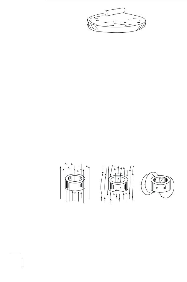
There is an interesting corollary to the Meissner e ect, which is the trapping of magnetic flux by a superconductor. Let us repeat our experiment demonstrating flux expulsion, but this time with a sample in the shape of a hollow cylinder. As the temperature is lowered through its critical value in the presence of the magnetic field, the flux lines are again expelled from the bulk of the material as expected. Nothing, however, comes in the way of the flux lines threading the hollow of the cylinder. Persistent screening currents will flow near the inner and the outer surfaces
(a) |
Hext ≠ 0 |
(b) |
Hext ≠ 0 |
(c) |
Hext = 0 |
N |
S |
S |
|
||
T > Tc |
T < Tc |
T < Tc |
Figure 3.5: Flux trapping by a hollow superconducting cylinder on field cooling.

3.4. Wholeness of Trapped Flux |
97 |
of the hollow cylinder as shown in Fig. 3.5. And now let us gradually remove the externally applied magnetic field leaving our sample all by itself. But what about the flux lines passing through the hollow of the cylinder? Surely they cannot escape sideways because in doing so they must traverse the surrounding superconducting material and this is forbidden by our perfect diamagnet — the flux is trapped. The persistent screening current now circulating near the inner surface of the hollow cylinder will sustain this trapped flux. What we have really got here is a permanent bar magnet. It is robust. You could carry it around in your pocket except for the inconvenience of having to keep it cold enough. Viewed di erently, you have created a non-polluting device for storing energy — the trapped magnetic flux and the circulating screening currents form a kind of flywheel, if you like, that stores (magnetic) energy at almost zero entropy.
3.4 Wholeness of Trapped Flux
The curious case of the trapped flux becomes all the more curious if we enquire further. What is the amount of magnetic flux trapped in the hollow of the cylinder? It turns out, and we will shortly know why, that the flux thus trapped cannot have an arbitrary value. It has to be an integral multiple of a certain basic unit of flux, denoted by φ0. That is to say that it must be a whole number when measured in lots of φ0. Fractions, or half-measures, are not allowed! This wholeness is the celebrated flux quantization, and φ0 the quantum of flux. This unit of flux is extremely small but still macroscopic enough. To have an idea of how small it is, imagine a circular wire loop of diameter 0.1 millimeter facing the earth’s magnetic field. Then the loop will intercept about 100 of these flux quanta! Small as it is, the trapped flux quanta can be counted by jiggling our cylinder in and out of a coil and then measuring the voltage (electromotive force) induced in the coil due to the changing flux linkages (Faraday’s law of induction). This was indeed done by B.S. Deaver and W.M. Fairbank in their classic experiment in 1961 that confirmed this quantization of trapped flux. As we shall see later, φ0 = hc/2e = 2 × 10⁻⁷ gauss centimeter-squared (= 2 ×10⁻¹⁵ tesla meter-squared) where h is Planck’s constant, c the speed of light and e the magnitude of the electric charge on the electron. Planck’s constant gives away the hidden quantum nature of superconductivity. It is a remarkable fact that the quantum nature of superconductivity was anticipated by Fritz London in 1935, long before the fully microscopic theory of superconductivity was given by John Bardeen, Leon N. Cooper and J. Robert Schrie er in 1957, the celebrated BCS theory for which the trio was awarded the Nobel Prize for Physics in 1972. In fact, London had predicted flux quantization, but being far ahead of his time, he missed the all important factor 2 in the denominator of φ0 = hc/2e. We now know after BCS that it is ‘2e’ and not ‘e,’ and thereby hangs the tale of ‘two electricities’ — the electron pairing theory of superconductivity.

98 |
Superconductivity |
3.5 Temperature and Phase Transition
The irresistible zero electrical resistance and the irrepressible infinite magnetic reluctance that set in at the critical temperature should leave us in no doubt that a qualitative change of state has taken place. There is a branch of physics that describes these changes of states of matter in general terms — thermodynamics, or statistical mechanics if we are interested in a microscopic treatment (see Appendix C). Temperature plays the central role here. This section is a brief digression intended to acquaint ourselves with some simple but powerful ideas that make the change of state understandable.
But first some quick remarks on the absolute (Kelvin) scale of temperature that we have already spoken of several times. Temperature is the intensity of heat. It measures the energy of the random jiggling of atoms, molecules, electrons, spins, or more generally, of the dynamical degrees of freedom that our system may have. Absolute temperature measures it absolutely. Thus, at the absolute zero of temperature the thermal energy is zero — all motion comes to a standstill. (There is, of course an irreducible zero-point motion even at the absolute zero of temperature which is of a purely quantum nature, and is appreciable for the so-called quantum liquids of which we will speak later. In fact, the superconductor is one such quantum liquid.) It is clear that any property that at all depends on temperature can be used to detect changes in temperature. Thus, the common household thermometer uses the thermal expansion of mercury for this purpose. One can also use, for example, the change of electrical resistance of metals, alloys or semiconductors to measure temperature charges. Thus, the Platinum (Pt) resistance thermometer is a prime standard for measuring temperatures down to −260◦C. But how can we meaningfully specify equal intervals of temperature? To say that equal changes in the length of the column of mercury in our thermometer give equal intervals of temperature is nothing more than an assertion that mercury expands equally for equal changes in temperature — clearly a circular statement empty of any objective content. For example, the equal intervals so defined may not be equal on a thermometer using alcohol instead of mercury. The question is if we can define equal intervals of temperature independently of the property of the material. The answer is Yes. As an act of almost pure reason, Lord Kelvin of Britain, one of the greatest of the classical physicists, proved in 1860 that such an absolute scale does exist and is defined in terms of the e ciency of an ideal heat engine. The absolute (or Kelvin) temperature scale (K) so defined is then conveniently graduated so that the boiling and the freezing points of water di er by 100 degrees on this scale just as on the commonly used centigrade scale (C) of Celsius. Then absolute zero (0 K) measures −273.15◦C and is the lowest temperature possible. Water freezes at 273.15 K (0◦C), and ‘room’ temperature is 300 K (26.85◦C). It is a profound result of classical statistical mechanics that every degree of freedom of a system such as a classical gas in equilibrium carries an equal amount of kinetic energy, kBT/2, where kB is the Boltzmann constant (the law of equipartition of energy).

3.5. Temperature and Phase Transition |
99 |
Temperature is the single most important control parameter that determines the states of matter. A solid (ice) melts to a liquid (water) and the liquid (water) boils to a gas (steam) as the temperature is raised through the well defined melting and the boiling points. These are the commonest and perhaps the most important changes of states that have shaped our biological lives and indeed the universe itself (see Chapter 10). Yet another interesting example of change of state is the loss of magnetization when a bar magnet is heated above its Curie temperature — the change from the ferromagnetic to the paramagnetic state. The change from the non-magnetic resistive normal state at high temperatures to the diamagnetic superconducting state at low temperatures is also a change of state, in fact closely related to the paramagnetic-to-ferromagnetic change of state. We call these di erent states di erent phases of the substance. The change of state is called phase transition, and the corresponding temperature the transition temperature.
3.5.1 Order Parameter
There is a feature which is common to all phase transitions. The higher temperature phase is disordered (or less ordered at any rate) while the lower temperature phase is ordered (or more ordered). There is indeed a competition between order and disorder, and temperature decides the winner. Thus, for example, the liquid state is disordered — a snap shot of the liquid state will show atoms positioned more or less at random, while the solid state formed upon freezing displays a periodic arrangement of atoms, which we call a crystal. Similarly, for the magnetic case, the spins (the tiny atomic magnets) point in di erent directions at random in the paramagnetic phase above the Curie temperature Tc, while they align parallel on average in the ferromagnetic phase below Tc. Indeed, one can define an order parameter that vanishes in the disordered phase but assumes a nonzero value in the ordered phase. For a magnet, the choice of the order parameter is obviously the magnetization. In the case of the superconducting transition, however, the nature of the order is too subtle as we will see later. The order parameter is one of the most powerful intermediate concepts in the physics of phase transition. It is an emergent quality. It was introduced by the great Russian physicist Leo Davidovich Landau in 1960, who gave a general theory of phase transition based on this crucial concept.
3.5.2 Free Energy and Entropy
What is the basic principle that determines which one of the possible phases our system in equilibrium will be found to be in? For mechanical systems with friction the answer is well known from our high school physics — the system will settle down to a state of minimum potential energy. Thus, a marble thrown in a bowl will eventually come to rest at the bottom-most point. This is a one-body problem. A somewhat similar minimum principle exists even for our many-body systems with

100 Superconductivity
a large, almost infinite number of particles (or degrees of freedom) interacting with one another. Left to itself, our system too will settle down to a final state which will change no more in time — a state of equilibrium. This state will, however, correspond to a minimum of what is called the free energy (see Appendix C). Let us see what this means. Consider a microscopic state of our system of energy E. A microscopic state means specifying in detail the momenta (roughly, velocities) and the positions of all the particles (degrees of freedom). Then, the energy E is the sum total of their kinetic and potential energies. Now, the fundamental principle of statistical mechanics is that all such microscopic states, which are possible at all, will occur, but with a probability proportional to exp(−E/kBT ). Next, strange as it may seem, almost all of these microscopic states of the same energy (E) look alike from the macroscopic (average) point of view. And it is the macroscopic viewpoint that matters for all practical purposes. (Indeed, even if we knew the finer microscopic details, we wouldn’t know what to do with them. The fact of the matter is that the microscopic description is too fine-grained while our usual probes are too coarse). Thus, for a given macroscopic state of energy E, there will be a large number of the microscopic states corresponding to the number of ways in which the energy E can be partitioned among the many degrees of freedom. Let this number be g(E). Hence, the probability of occurrence of the physically identifiable macroscopic state must be proportional to g(E) times exp(−E/kBT ). We may re-write this as exp(−F/kBT ) with the exponent F = E − kBT ln[g(E)]. Here ln[g] denotes the ‘natural’ logarithm of g with respect to base e = 2.71828 . . . .
So the most probable state is the one that corresponds to the minimum of F , the Free Energy and not of E. The quantity kB ln[g(E)] is the mysterious entropy and is usually denoted by S. Thus, we must minimize F = E − T S, and not just E. At T = 0 K, this, of course, reduces to minimizing the energy itself. This lowest energy state, called the ground state, is essentially unique for the system. For this state, g is unity and hence S = 0 (remember, the logarithm of unity = 0). The ground state, the most ordered state, has zero entropy! It is clear that at a su ciently high temperature the entropy term in F may dominate the free-energy and a di erent state may be preferred. In general, g(E) and, therefore, entropy is expected to increase with energy — there are then obviously more ways of partitioning it among the various degrees of freedom. The corresponding macroscopic state will also be more disordered. Ordered microscopic states are fewer due to the constraints of order, and hence the corresponding ordered macroscopic state has lower entropy. (Just compare the disorderly crowd and the disciplined military and you will have the general drift of the idea.) And so it happens that high temperature favors disorder. The relationship between the many microscopic states and the single macroscopic state corresponding to them is illustrated best by an analogy with the game of dice. Consider casting two dice simultaneously. Each can come face-up with a number from 1 to 6. Thus there are 6 × 6 = 36 possibilities. These are all the possible 36 microscopic states of our system of the two dice. Let the dice

3.6. Type I Superconductors |
101 |
be true for simplicity. Then all 36 microscopic states are equally probable. But suppose now that we are interested only in the sum of the numbers that the two dice come up with. The sum can vary from 1 + 1 = 2 to 6 + 6 = 12. These are then the 11 macroscopic states. Let us label them by the sums 2 to 12. Now you see that the macroscopic state 2 = 1 + 1 is realized in only one way, and the macroscopic state 3 = 1 + 2 = 2 + 1 in two ways, and so on. You can easily verify that the macroscopic state 7 is realized in six ways, which is the maximum and hence the most probable state. If you want to push this analogy further then all you have to do is to imagine a large, almost infinite number of dice, and let the dice not be true. Then the most probable macrostate is all that will occur overwhelmingly. The others may be regarded as mere fluctuations about this. But a discussion of these fluctuations will take us far afield.
In the case of our superconducting material the fact that for T < Tc, the material is in the superconducting (S) state implies that it has a free-energy less than the normal (N) state. The di erence FN −FS is called the condensation free energy and is denoted by ∆F . (The corresponding ∆E is the condensation energy.) It is clear that ∆F is positive and a maximum at 0 K, falls o to zero at T = Tc and then turns negative for T > Tc when the normal state takes over.
Calculating the free energy is a horrendous task of statistical mechanics. But the principle of phase transition is now clear. The behavior of free energy determines the nature of the phase transition. It may be a discontinuous one, where the energy E changes by a finite amount even though F is (as it must be) continuous. This discontinuous change of E is the latent heat that is given out (absorbed) during freezing (melting) or condensation (boiling). We have all experienced it some time or the other, rather regretfully though — the scalding of the hand exposed to condensing steam from a boiling pot. We call these first-order phase transitions. The superconducting transition, on the other hand, is a continuous transition with no latent heat associated with it. The same is true of the magnetic transition. These are called second-order phase transitions. Unlike first-order transitions, the changes that take place at and near the second-order phase transition are very subtle. Several physical quantities, such as the specific heat, show singular behavior which is remarkably universal.
3.6 Type I Superconductors
While superconductors are all alike electrically, namely that they all transport electricity without loss once they are below the critical temperature and at very low currents, their magnetic behavior can be really very di erent. The perfect diamagnetism that we have spoken of typifies a superconductor of Type I. Their behavior is understood quite simply. Expulsion of the magnetic field from the bulk of the superconductor requires doing some work against the magnetic pressure of the field thus expelled. It is like blowing up a balloon. You may picture the magnetic

102 |
Superconductivity |
H
S
λL
Figure 3.6: Flux penetration in a superconductor (S). The London penetration length λL.
lines of force as elastic strings under tension. They get stretched as they are pushed out sideways (Fig. 3.3). The amount of work done on the system is proportional to the square of the field H. This raises the energy (and, therefore, the free energy) of the superconductor by the same amount. It is clear now that when this exceeds the condensation energy, the superconducting state will no longer be favorable energetically and the sample will turn normal. This defines a critical field Hc such that superconductivity prevails only for H < Hc. Inasmuch as the condensation energy decreases from a maximum at T = 0 K to zero at T = Tc, Hc too will behave likewise. Typical examples of a Type I superconductor are mercury, aluminum and tin. The critical field Hc is typically 0.1 tesla (1 kilogauss).
Even below Hc, the flux expulsion is really only partial. Indeed, it is energetically favorable to allow the field to penetrate some distance into the interior of the sample. This is a kind of energy minimization through an optimal compromise as we shall see later. In fact the field diminishes exponentially as exp(−x/λL) with the depth x below the surface of the sample (Fig. 3.6). The characteristic length λL is called the London penetration depth. The screening currents flow mainly within this depth.
2 3 ˚ ˚ −8
For the Type I superconductors, λL is typically 10 –10 A (1 A = 10 cm). It is smallest at 0 K and grows to infinity (i.e., the size of the sample) as we approach Tc, where the sample turns normal and is filled with the flux lines uniformly.
3.7 Type II Superconductors
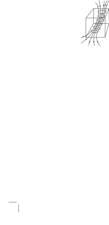
Type II superconductors are di erent, and much more interesting. Discovered in 1937 by the Russian physicist L. V. Shubnikov, they are also the more important of the two types for most practical applications. They show the Meissner e ect just like Type I superconductors up to a lower critical field Hc1. As the magnetic field exceeds Hc1, something catastrophic happens: the flux rushes into the bulk of the superconductor and permeates the whole sample. But it does so in the form of filaments, or flux tubes, rather than uniformly (Fig. 3.7). Each flux-tube carries exactly one quantum of flux. As the external field is increased, more and more flux tubes are formed in the sample to accommodate the increased total flux. This goes on until the flux tubes begin to almost touch each other at H = Hc2, the upper critical field, beyond which superconductivity is destroyed. For Type II superconductors, the upper critical field Hc2 is typically 1 to 10 tesla (10–100 kilogauss).
3.7. Type II Superconductors |
103 |
S
0
Figure 3.7: Flux tube in a superconductor (S) carrying single flux quantum φ0.
The flux tubes are very real. You can make them visible by sprinkling finely divided iron filings on the surface of the superconductor. The iron filings naturally cling to the foot points where the flux-tubes emerge from the superconductor and thus give them away. Such flux decoration experiments demonstrate not just the existence of the flux tubes, but also that these flux tubes are ordered in space as a triangular lattice at low temperatures. This is the so-called Abrikosov flux lattice, named after the Russian physicist A.A. Abrikosov who predicted it theoretically in 1957. The flux lattice is very real. It can vibrate elastically and even melt at higher temperatures and form a flux liquid, where the flux tubes can get entangled like the strands of melted polymers and hinder their mobility.
An individual flux tube has an interesting structure. It has a core which is in the normal state in that the superconducting order-parameter (or the condensation energy) is locally depressed to zero. The e ect of this depression extends out to a distance ξ from the axis of the tube. This is the so-called coherence length and measures the distance over which the superconducting order is correlated — it is the minimum distance over which the superconducting order can change appreciably. Such a coherence is characteristic of all systems ordered one way or another. Thus, the superconducting order-parameter (roughly the condensation energy), which is zero in the normal core, will rise to its full value only beyond ξ, in the superconducting regions between the flux tubes. The magnetic field, on the other hand, will have its maximum value along the axis in the core region, and will fall o to almost zero beyond a distance λL away from the axis. Surrounding the core we will have the circulating supercurrents that do this screening of the field. Thus, the flux tube looks like a vortex and this state for Hc1 < H < Hc2 is called the vortex state. Here the normal core region co-exists with superconducting regions intervening between the cores. For this reason the vortex state is also called the mixed state.
Let us see now what determines the type of a superconductor. The basic principle is the same — the free energy must be minimized. For a superconductor this requires compromise between two competing tendencies that operate at the interface (or the

104 |
Superconductivity |
boundary) between the superconducting region of the sample and the region driven normal by the magnetic field. On the one hand it is favorable energetically to let the magnetic field penetrate the superconducting region and thereby reduce the energy cost of flux expulsion. This gain in energy is proportional to the London penetration depth λL for a given area of the interface. On the other hand, the superconducting order (or the condensation energy), which is depressed to zero in the core, remains more or less depressed up to a distance ξ from the axis of the flux tube. This costs energy proportional to ξ for the given area of the interface. Thus, for ξ much greater than λL, it is energetically favorable to reduce the total area of the interface. It is as if there is a positive interfacial surface energy per unit area (a surface tension). This will correspond to a complete Meissner e ect — total expulsion of flux as in a Type I superconductor. For the opposite case of ξ much less than λL, it is energetically favorable to increase the interface area as if the surface tension is negative. This is realized by flux tubes filling the sample as in a Type II superconductor. Detailed calculation shows that ξ λL is the dividing line. The basic physics here is the same as that of wetting — water wets glass while mercury does not wet it. A more closely related situation is that of mixing of oil and water in the presence of some surfactant that controls surface tension. The mixture may phase-separate into water and oil (Type I) or, globules of oil may be interspersed in water (Type II). The Type II superconductor is indeed a laboratory for doing interesting physics.
3.8The Critical Current
The critical field (Hc for Type I or Hc2 for Type II) is an important parameter that limits the current carrying capacity of a superconductor. This is because a superconducting wire carrying current generates its own magnetic field (Ampere’s Law) and if this self-field exceeds Hc or Hc2, superconductivity will be quenched. This defines a critical current density, Jc. Clearly, a Type II superconductor with large Hc2 up to 10 teslas, is far superior to Type I superconductors with Hc of about 0.1 tesla. There is, however, a snag here that involves some pretty physics. Consider a flux tube threading a Type II superconductor, and let an electric current I flow perpendicular to the flux tube. Now, by the Faraday principle of the electric motor, there will be a force acting on the flux tube, forcing it to move sideways perpendicular to the current and proportional to it. Physicists call it the Lorentz force. Once the flux tube starts moving with some velocity, the Faraday principle of the electric generator (the dynamo principle of flux cutting) begins to operate — an electromotive force (potential drop, V ) is generated perpendicular to both the flux tube as well as its velocity so as to oppose the impressed current, I. This leads to dissipation of energy. Remember W (watts) = V (voltage drop) × I (amperes). We have the paradoxical situation of having a lossy superconductor! Where is the energy dissipated, you may ask. Well, the core of the flux tube is in the normal state