

Measurement and Control Basics 3rd Edition (complete book)
.pdfChapter 2 – Process Control Loops |
45 |
|
|
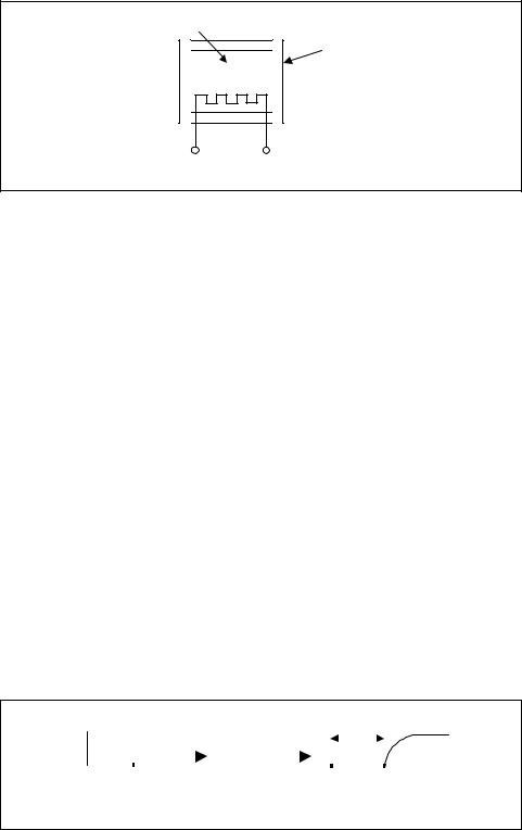
Insulation |
Heat in, q |
C |
To = Ambient Temperature |
|
||
|
|
Body of mass, M, |
|
|
with Thermal |
|
|
Capacitance, C |
Figure 2-12. Thermal capacitance |
|
|
The rate of heat flow through a body is determined by its thermal resistance. This is defined as the change in temperature that results from a unit change in heat flow rate. Thermal resistance is normally a linear function, in which case,
RT |
= |
T2 − T1 |
(2-37) |
|
q |
||||
|
|
|
where
RT |
= thermal resistance (°C/ cal/s) |
T2 - T1 = temperature difference in (°C)
q |
= the heat flow (cal/s) |
Thermal resistance is analogous to the resistance in an electrical circuit.
If the temperature of a body is considered to be uniform throughout, its thermal behavior can be described by a linear differential equation. This assumption is generally true for small bodies of gases or liquids where perfect mixing takes place. For such a system, thermal equilibrium requires that at any instant the heat added (qi) to the system equals the heat stored (qs) plus the heat removed (qo). Thus,
qi = qs + qo |
(2-38) |
Table 2-1 compares variables in the three different physical systems we have discussed. It is important to have a general idea of the physical meaning of process time constants so you can observe a process with some understanding of its capacity to store material or energy. In this way, you can gain some insight into the process dynamics of a system. Such an understanding is very important in process control design.

46 Measurement and Control Basics
EXAMPLE 2-3
Problem: Derive the differential equation for the water temperature, TW, for an insulated tank of water that is heated using an electric heater as shown in Figure 2-13. Assume that the rate of heat flow from the heating element is qi and that the water is at a uniform temperature. Also assume that no heat is stored in the insulation.
Solution: Using Equation 2-35, the heat stored in the water is as follows:
qw = C dT dt
where C is the thermal capacitance of the water. From Equation 2-37, the heat loss through the insulation is the following:
q o |
= |
TW − To |
|
R |
|||
|
|
where To is the temperature of the air outside the tank. Applying Equation 2-38 yields
|
qi = qs + qo |
|
|||
or |
|
|
|
|
|
qi |
= C |
dTW |
+ |
TW − To |
|
|
|
||||
|
|
dt |
R |
||
By multiplying this equation by R and allowing the system constant (τ) tο replace the term RC, we obtain
Rqi = RC dTW + TW − To
dt
or
RC dTW + TW = To + Rqi
dt
If we replace RC with the time constant symbol, τ , we obtain
τ |
dTW |
+ T |
= T |
+ Rq |
|
|
i |
||||
|
dt |
W |
o |
|
|
|
|
|
|
|
which is a first-order differential equation for water temperature TW.
Chapter 2 – Process Control Loops |
47 |
Tw , Water Temperature
Heater |
Insulation with Thermal Resistance, R
To , Air Temperature
Power In
Figure 2-13. Thermal system for Example 2-3
Table 2-1. Comparison of Physical Units
Variable |
|
System Type |
|
|
|
|
|
||
Electrical |
Liquid |
Thermal |
||
|
||||
|
|
|
|
|
Quantity |
Coulomb (c) |
Cubic meter (m3) |
cal |
|
|
|
|
|
|
Potential |
Volt (v) |
meter (m) |
°C |
|
|
|
|
|
|
Flow |
Ampere (A) |
m3/s |
cal/s |
|
|
|
|
|
|
Resistance |
Ohms (Ω ) |
m/m3/s |
°C/cal/s |
|
|
|
|
|
|
Capacitance |
Farad (F) |
m/m3 |
cal/°C |
|
|
|
|
|
|
Time |
Second (s) |
Second (s) |
Second (s) |
|
|
|
|
|
Dead Time Lag
In general, not all processes can be neatly characterized by first-order lags. In some cases, a process will produce a response curve like that shown in Figure 2-14. In this process, the maximum rate of change for the output does not occur at time zero (to) but at some later time (t1). This is called dead time in process control: the period of time (td) that elapses between the moment a change is introduced into a process and the moment the output of the process begins to change. Dead time is shown in Figure 2-14 as the time between t1 and to, or td = t1 - to.
|
|
|
|
|
|
|
|
|
|
|
|
|
|
td |
|
|
|
|
|
|
|
|
|
|
|
|
|
|
|
|
|
|
|
|
|
|
|
|
|
|
|
|
|
Process |
|
|
|
|
|
|
|
|
|
|
|
|
t1 |
|
|
|
|
|
|
|
|
|
|
|
|
||
t0 |
|
|
|
|
|
|
|
|
|
|
|
|
|
||||
|
|
|
|
|
|
t0 |
|
|
t1 |
||||||||
|
|
|
|
|
|
|
|
||||||||||
Step Input |
|
|
|
|
|
Output Response |
|||||||||||
Figure 2-14. Dead time response to step input
48 Measurement and Control Basics
Dead time is the most difficult condition to overcome in process control. During dead time, there is no process response and therefore no information available to initiate corrective action.
To illustrate the concept of dead time, consider the temperature feedback control system shown in Figure 2-15. In this process, steam is used to heat process fluid that is used in other parts of a plant. A temperature detector in the heat exchanger discharge line measures the temperature of the process fluid. The control system increases or decreases the steam into the heat exchanger to maintain the outlet fluid at a desired temperature.
IA |
TY |
I/P |
TIC |
|
|
|
|||
100 |
|
100 |
|
|
|
|
|
||
|
|
TV |
|
|
|
|
100 |
|
|
Steam |
|
|
TT |
TE |
|
|
100 |
100 |
|
Process |
|
|
|
Process |
Fluid |
|
|
D |
Fluid |
|
|
|
|
|
|
|
E-100 |
Condensate |
|
|
|
|
|
|
Figure 2-15. Dead time in control loop |
|
|
||
In the design of this control loop, the location of the temperature detector is critical. It is tempting to say that the detector should be installed farther down the outlet pipe and closer to the point at which the process fluid is used. This seems correct because the temperature of the process fluid in the heat exchanger or at the discharge point of the exchanger is of little importance to the user of the heated process fluid. However, this line of reasoning can be disastrous because as the detector is moved farther and farther down the line, a larger and larger dead time is introduced. In the example in Figure 2-15, the process dead time (td) is equal to the distance (D) between the heat exchanger and the temperature sensor, divided by the velocity (v) of the water flowing through the discharge pipe, or
td = D/v. If excessive dead time is introduced into this temperature control loop, the loop performance will deteriorate and may reach a point where it is impossible to achieve stable control.
An example will aid in understanding dead time in a typical process.

Chapter 2 – Process Control Loops |
49 |
EXAMPLE 2-4
Problem: Determine the dead time for the process shown in Figure 2-15 if the temperature detector is located 50 meters from the heat exchanger and the velocity of the process fluid in the discharge pipe is 10 m/s.
Solution: The dead time is given by td = D/v. Since D = 50 m and v = 10 m/s
td |
= |
D |
= |
50 m |
= 5 s |
|
|
||||
|
|
v |
10 m/s |
||
Dead time occurs in many types of processes, and it is the most difficult process condition to correct for in control applications. You can detect process dead time from a process response curve by measuring the amount of time that elapses before any output response occurs after an input change is applied to a system. Process reaction curves are discussed in a later section of this chapter.
Advanced Control Loops
Up to this point, we have discussed only single-loop feedback control. This section will now expand the discussion to include cascade, ratio, and feedforward control loops.
Cascade Control Loops
The general concept of cascade control is to place one feedback loop inside another. In effect, one takes the process being controlled and finds some intermediate variable within the process to use as the set point for the main loop.
Cascade control exhibits its real value when a very slow process is being controlled. In such circumstances, errors can exist for a very long time, and when disturbances enter the process there may be a significant wait before any corrective action is initiated. Also, once corrective action is taken one may have to wait a long time for results. Cascade control allows the operator to find intermediate controlled variables and to take corrective action on disturbances more promptly. In general, cascade control offers significant advantages and is one of the most underutilized feedback control techniques.
An important question you may confront when implementing cascade control is how to select the most advantageous secondary controlled vari-
50 Measurement and Control Basics
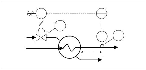
able. Quite often, the designer has a large number of choices. The overall strategy or goal should be to get as much of the process lag into the outer loop as possible while, at the same time, getting as many of the disturbances as possible to enter the inner loop.
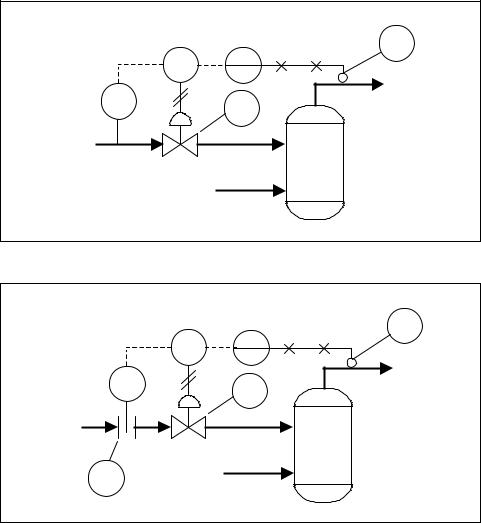
Figures 2-16 and 2-17 illustrate two different cascade control arrangements for a furnace that is used to increase the temperature of a fluid that is passing through it. In both cases, the primary controlled variable is the same, but in each case a different intermediate controlled variable has been selected. The question then is which type of cascade control is best.
|
|
TE |
PIC SP |
TIC |
100 |
|
||
100 |
100 |
Out |
PT |
|
|
PV |
|
|
100 |
|
|
100 |
|
|
|
|
|
Fuel |
|
|
|
|
Furnace |
In |
|
|
Figure 2-16. Pressure and temperature cascade control
|
|
TE |
FIC |
SP TIC |
100 |
100 |
100 |
Out |
FT |
|
|
FV |
|
|
100 |
|
|
100 |
|
|
|
|
|
Fuel |
|
|
|
|
Furnace |
FE |
In |
|
100 |
|
|
Figure 2-17. Flow and temperature cascade control
Chapter 2 – Process Control Loops |
51 |
To determine the best cascade control arrangement, you must identify the most likely disturbances to the system. It is helpful to make a list of these in order of increasing importance. Once this has been done, the designer can review the various cascade control options available and determine which one best meets the overall strategy outlined earlier: to make the inner loop as fast as possible while at the same time receiving the bulk of the important disturbances.
If both controllers of a cascade control system are three-mode controllers, there are a total of six tuning adjustments. It is doubtful that such a system could ever be tuned effectively. Therefore, you should select with care the modes to be included in both the primary and secondary controllers of a cascade arrangement.
For the secondary (inner or slave) controller, it is standard practice to include the proportional mode. There is little need to include the reset mode to eliminate offset because the set point for the inner controller will be reset continuously by the outer or master controller. For the outer loop, the controller should contain the proportional mode. If the loop is sufficiently important to merit cascade control then you should probably include reset to eliminate offset in the outer loop. You should undertake rate or derivative control in either loop only if it has a very large amount of lag.
The tuning of cascade controllers is the same as the tuning of all feedback controllers, but the loop must be tuned from the inside out. The master controller should be put on manual (i.e., the loop broken), and then the inner loop can be tuned. Once the inner loop is properly tuned, the outer loop can be tuned. This allows the outer loop to “see” the tuned inner loop functioning as part of the total process or as the “all else” that is being controlled by the master controller. If you follow this general inside-first principle when tuning cascade controllers, you should encounter no special problems.
Ratio Control Loops
Another common type of feedback control system is ratio control. Based on hardware, ratio control is quite often confused with cascade control. The basic operation of ratio control, however, is quite different.
Ratio control is often associated with process operations in which two or more streams must be mixed together continuously to maintain a steady composition in the resulting mixture. A practical way to do this is to use a conventional flow controller on one stream and to control the other stream with a ratio controller that maintains flow in some preset ratio or fraction
52 Measurement and Control Basics
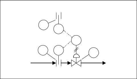
to the primary stream flow. A preset ratio regulates the flow of the controlled variable. For example, if the ratio is 10 to 1, then for every gallon per minute of the uncontrolled variable that is flowing, ten gallons per minute of the controlled variable are allowed to flow. A typical ratio control system is shown in Figure 2-18.
Uncontrolled Flow
Air 
 Air
Air
FE |
|
|
|
200 |
FT |
|
|
|
200 |
SP |
|
|
|
|
|
|
|
FFIC |
|
|
|
100 |
|
FE |
FT |
PV |
|
|
FV |
||
100 |
100 |
|
|
|
100 |
||
|
|
|
|
Fuel |
|
|
Fuel |
|
Controlled Flow |
|
|
Figure 2-18. Ratio control
Use the signal from the uncontrolled flow transmitter, or wild flow, as the ratio input of the ratio controller. Multiply the value by an adjustable factor or ratio setting to determine the set point of the flow controller. The process variable to the controller is the flow of the controlled stream. The output from the ratio controller adjusts the control valve.
You can use a ratio control loop with any combination of suitably related process variables, and the control action selected is normally proportional plus integral. The response to process upsets of a control loop with ratio control is the same as the response found in a single-feedback loop.
Feedforward Control Loops
A feedback control loop is reactive in nature and represents a response to the effect of a load change or upset. A feedforward control loop, on the other hand, responds directly to load changes and thus provides improved control.
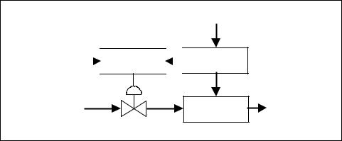
In feedforward control, a sensor is used to detect process load changes or disturbances as they enter the system. A block diagram of a typical feed-
Chapter 2 – Process Control Loops |
53 |
forward control loop is shown in Figure 2-19. Sensors measure the values of the load variables, and a computer calculates the correct control signal for the existing load conditions and process set point.
Load Changes
Set Point 
 Feedforward
 Measurement
Calculation
Input |
Process |
Output |
Control Valve
Figure 2-19. Feedforward control
Feedforward control poses some significant problems. Its configuration assumes that the disturbances are known in advance, that they will have sensors associated with them, and that no important undetected disturbances will occur.
Therefore, feedforward control is more complicated and more expensive, and it requires the operator to have a better understanding of the process than does a standard feedback control loop. So, feedforward control is generally reserved for well-understood and critical applications.
Tuning Control Loops
There are three important factors to consider when tuning a PID controller: the characteristics of the process, the selection of controller modes, and the performance criteria of the control loop.
Selecting Controller Modes
Which controller mode to select is an important consideration when tuning controllers. Four basic control combinations are used: proportional only, proportional plus integral (PI), proportional plus derivative (PD), and proportional plus integral plus derivative (PID).
The most basic continuous control mode is proportional control. Here, the controller output (m) is algebraically proportional to the error (e) input

54 Measurement and Control Basics
signal to a controller. The equation for proportional control is given by the following equation:
m = K c e |
(2-39) |
This equation is also called the proportional control algorithm. This control action is the simplest and most commonly encountered of all the continuous control modes. In effect, there is a continuous linear relationship between the controller input and output.
The proportional gain of the controller is the term Kc, which is also referred to as the proportional sensitivity of the controller. Kc indicates the change in the manipulated variable per unit change in the error signal. In a true sense, the proportional sensitivity or gain is a multiplication term. It represents a parameter on a piece of actual hardware that must be adjusted by a technician or engineer; for example, the gain may be an adjustable knob on the process controller.
On many industrial controllers, this gain-adjusting mechanism is not expressed in terms of proportional sensitivity or gain but in terms of proportional band (PB). Proportional band is defined as the span of values of the input that corresponds to a full or complete change in the output. This is usually expressed as a percentage. It is related to proportional gain by the following equation:
= 100%
PB (2-40)
K c
Most controllers have a scale that indicates the value of the final controlled variable. Therefore, the proportional band can be conveniently expressed as the range of values of the controlled variable that corresponds to the full operating range of the final control valve. As a matter of practice, wide bands (high percentages of PB) correspond to less sensitive response, and narrow bands (low percentages) correspond to more sensitive response of the controller.
Proportional control is quite simple and is the easiest of the continuous controllers to tune since there is only one parameter to adjust. It also provides very rapid response and is relatively stable. Proportional control has one major disadvantage, however: at steady state, it exhibits offset. That is, there is a difference at steady state between the desired value or set point and the actual value of the controlled. To correct for this problem proportional control is combined with integral action.