

Measurement and Control Basics 3rd Edition (complete book)
.pdfChapter 7 – Temperature Measurement |
195 |
where |
|
|
T |
= |
temperature (K) |
R |
= |
resistance (Ω) of the thermistor |
A, B, and C |
= |
curve-fitting constants |
You can find the constants A, B, and C by selecting three data points on the published data curve and solving the three simultaneous equations. When you choose data points that span no more than 100°C within the nominal center of the thermistor's temperature range, this equation approaches a remarkable +0.01°C curve fit.
Example 7-8 illustrates a typical calculation to obtain the temperature for a thermistor with a known resistance.
A great deal of effort has gone into developing thermistors that approach a linear characteristic. These are typically threeor four-lead devices that require the use of external matching resistors to linearize the characteristic curve. Modern data acquisition systems with built-in microprocessors have made this type of hardware linearization unnecessary.
The high resistivity of the thermistor affords it a distinct measurement advantage. The four-wire resistance measurement is not required as it is with RTDs. For example, a common thermistor value is 5,000 Ω at 25°C. With a typical temperature coefficient of 4%/°C, a measurement lead resistance of 10 Ω produces only a 0.05°C error. This is a factor of five hundred times less than the equivalent RTD error.
Because thermistors are semiconductors, they are more susceptible to permanent decalibration at high temperatures than are RTDs or thermocouples. The use of thermistors is generally limited to a few hundred degrees Celsius, and manufacturers warn that extended exposures, even well below maximum operating limits, will cause the thermistor to drift out of its specified tolerance.
Thermistors can be manufactured very small, which means they will respond quickly to temperature changes. It also means that their small thermal mass makes them susceptible to self-heating errors. Thermistors are more fragile than RTDs or thermocouples, and you must mount them carefully to avoid crushing or bond separation.
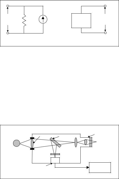
Integrated-Circuit Temperature Sensors
Integrated-circuit temperature transducers are available in both voltage and current-output configurations (Figure 7-20). Both supply an output

196 Measurement and Control Basics
EXAMPLE 7-8
Problem: A typical thermistor has the following coefficients for the SteinhartHart equation:
A = 1.1252 × 10⁻³/K
B = 2.3478 × 10⁻⁴/K
C = 8.5262 × 10⁻⁸/K
Calculate the temperature when the resistance is 4000 Ω .
Solution: Using Equation 7-11, we obtain the following:
1 = A + B ln R + C(ln R)3
T
1 =1.1252x10⁻³ / K + (2.3478x10⁻⁴ / K )(ln 4000) + (8.5262x10⁻⁸ / K )(ln 4000)3
T
1 =1.1252x10⁻³ / K +1.9471x10⁻³ / K + 0.0486x10⁻³ / K T
1 = 3.1209x10⁻³ / K T
T = 320.4 K
Now convert from Kelvin to Celsius:
T = (320.4 – 273.15)°C
T = 47.25°C
that is linearly proportional to absolute temperature. Typical values are one microampere of current per one-degree temperature change in Kelvin (1 A/K) and ten millivolts per one-degree change in Kelvin (10 mv/K).
Except for the fact that these devices provide an output that is very linear with temperature, they share all the disadvantages of thermistors. They are semiconductor devices and thus have a limited temperature range. Integrated-circuit temperature sensors are normally only used in applica-
Chapter 7 – Temperature Measurement |
197 |
+ |
|
|
+ |
DVM |
1 A/K |
10 mV/K |
DVM |
_ |
|
|
_ |
a) Current - IC Temperature Sensor |
b) Voltage - IC Temperature Sensor |
||
Figure 7-20. Integrated-circuit temperature transducers
tions that have a limited temperature range. One typical application is in temperature data acquisition systems where they are used for thermocouple compensation.
Radiation Pyrometers
A pyrometer is any temperature-measuring device that includes a sensor and a readout. However, in this section we will discuss only radiationtype pyrometers. A radiation pyrometer is a noncontact temperature sensor that infers the temperature of an object by detecting its naturally emitted thermal radiation. An optical system collects the visible and infrared energy from an object and focuses it on a detector, as shown in Figure 7-21. The detector converts the collected energy into an electrical signal to drive a temperature display or control unit.
|
|
|
Adjustable |
Hot Object |
Len |
Mirror |
Eyepiece |
|
|
|
|
|
Detector |
|
Temperature |
|
|
|
Indicator |
Figure 7-21. Block diagram of radiation pyrometer
198 Measurement and Control Basics
The detector receives the photon energy from the optical system and converts it into an electrical signal. Two types of detectors are used: thermal (thermopile) and photon (photomultiplier tubes). Photon detectors are much faster than the thermopile type. This enables you to use the photon type for measuring the temperature of small objects moving at high speed.
Radiation pyrometers are used to measure the temperature of very hot objects without being in contact with them. Molten glass and molten metals during smelting and forming operations are typical of the objects they measure. In selecting the correct radiation pyrometer for an application you must consider several factors. In either narrow or wide fields of view, the cross-sectional area can vary greatly. It can be rectangular, circular, and slot shaped, depending on the kind of apertures used in the instrument. In some instruments, a telescopic eye magnifies the radiant energy so much smaller objects at longer distances can be measured. Hot objects as small as 1/16 inch in diameter can be measured with some instruments.
The construction of the instrument components, such as the lens and curved mirrors, control the sight path. The materials of construction determine the optical characteristics of the device. For example, glass does not transmit light well beyond 2.5 microns. It is therefore suitable only for high-temperature applications where high-energy outputs are present. Other common optical materials are quartz (transmitting well to 4 microns) and crystalline calcium fluoride (transmitting well up to about 10 microns). Band pass filters are used in some instruments to cut off unwanted light at certain wavelengths.
EXERCISES
7.1Express a temperature of 133°C in both °F and Kelvin.
7.2Express a temperature of 400 °F in both °C and Kelvin.
7.3A gas in a fixed-volume temperature sensor has a pressure of 21 psia at a temperature of 25°C. What is the temperature in °C if the pressure in the detector increases to 22 psia?
7.4How much will a 10-m-long copper rod at 20°C expand when the temperature is changed from 0 to 100°C?
7.5List the normal operating ranges for J-, K-, and S-type thermocouples.
7.6Find the Seebeck voltage for a TC with α = 36 µv/°C if the junction temperatures are 25°C and 75 °C.
7.7A voltage of 10.10 mv is measured across a type K thermocouple at a 0 °C reference. Find the temperature at the measurement junction.
Chapter 7 – Temperature Measurement |
199 |
7.8A voltage of 19.50 mv is measured across a type J thermocouple at a 0 °C reference. Find the temperature at the measurement junction.
7.9Explain the purpose and function of the isothermal blocks in a digital voltmeter temperature-measuring circuit.
7.10Calculate the resistance ratio for a platinum RTD with α = 0.00392 and δ = 1.49 when T = 80 °C.
7.11Calculate the temperature measured by a thermistor when the resistance is 2,800 Ω . Assume that the thermistor has the following coefficients for the Steinhart-Hart equation: A = 1.1252 X 10⁻³/K, B = 2.3478 X 10⁻⁴/K, and C = 3.5262 X 10⁻⁸/K.
BIBLIOGRAPHY
1.Hall, J. (ed.). “Sensor/Transducer Course,” Instruments & Control Systems, 1990.
2.Halliday, D., and R. Resnick. Physics for Students of Science and Engineering,
New York: John Wiley & Sons, 1963.
3.Hewlett-Packard Company. Practical Temperature Measurement-Applications Note 290, 1987, Hewlett Packard Company.
4.Johnson, C. D. Process Control Instrumentation Technology, 2d ed., New York: John Wiley & Sons, 1982.
5.Liptak, B. G., and D. Venczel (ed.). Process Control—Instrument Engineers Handbook, rev. ed., Radnor, PA: Chilton.
6.Omega Engineering. Temperature Measurement Handbook 1986, Stanford, CT: Omega Engineering.

8
Analytical Measurement and Control
Introduction
This chapter discusses the basic principles of chemical analytical measurement and control, with an emphasis on the following areas: conductivity, pH, density, humidity, turbidity, and gas analysis. We introduce the basic principles of electromagnetic (EM) radiation and describe several common phototransducers that use EM radiation to measure analytical variables.
Conductivity Measurement
Measuring conductivity means determining a solution's ability to conduct electric current. This ability is referred to as specific conductance—or, simply, conductivity—and is expressed in “mhos,” which is the reciprocal of ohm (the unit used to express resistance).
Aqueous solutions of acids, bases, or salts are known as electrolytes; they are conductors of electricity. Conductivity measurements are generally made to detect electrolytic contaminants around water and waste-treat- ment areas. The degree of electrical conductivity of such solutions is affected by three factors: the nature of the electrolyte, the concentration of the solution, and the temperature of the solution. A measurement of the conductivity at a fixed temperature can be a measurement of the solution's concentration, which can be expressed in percentage terms by weight, parts per million, or other applicable units.
If you know the conductivity values of various concentrations of an electrolyte, you can then determine the concentration by passing current
201

202 Measurement and Control Basics
through a solution of known dimensions and measuring its electrical resistivity or conductivity.
The primary element in an electrical conductivity system is the conductivity cell (see Figure 8-1). Such cells consist of a pair of electrodes whose areas and spacing are precisely fixed, a suitable insulating member to confine the conductive paths, and suitable fittings for supporting and protecting the cell. The conductance between two electrodes varies as follows:
|
|
|
|
|
|
|
|
|
|
|
|
|
|
|
A |
(8-1) |
|
|
|
|
|
|
|
|
|
|
|
|
C∞ --- |
||||
|
|
|
|
|
|
|
|
|
|
|
|
|
|
|
L |
|
where |
|
|
|
|
|
|
|
|
|
|
|
|
|
|
|
|
C |
= conductance (mho) |
|
||||||||||||||
A |
= the area of electrodes (cm2) |
|
||||||||||||||
L |
= the distance between electrodes (cm) |
|
||||||||||||||
|
|
|
|
|
|
|
|
|
|
|
|
|
|
|
|
|
To Wheatstone
Bridge Circuit
Area (A)
Electrodes
L
Figure 8-1. Conductivity cell
To establish a common basis for comparing conductivities of different solutions, a standard conductivity cell is considered for which the following is true:
A = 1 cm2
L = 1 cm
This volume of solution is completely insulated from its surroundings. Unless this insulated condition is met, no simple relationship exists between conductance and A/L. This is because there are additional conducting paths available between electrodes. This conductance of the solution in a unit cell is called its specific conductivity k (sometimes called

Chapter 8 – Analytical Measurement and Control |
203 |
conductance) and has units of mhos per centimeter (mho/cm). In common practice, the specific conductance in mhos per centimeter is referred to as the solution's “conductivity” and is given in units of mhos only. For example, an electrolyte with a specific conductance of 0.03 mho/cm is said to have a conductivity of 0.03 mho. The two terms are synonymous as they are commonly used.
Conductivity instruments normally use some variation of an AC Wheatstone bridge circuit to measure solution conductivity. Alternating current is used to eliminate electrode polarization effects. Using platinum electrodes can further reduce these effects. Conductivity analyzers generally use an AC frequency of 50 to 600 Hz, and the normal range of resistance measured is from 100 to 60,000 W.
The instrument can be calibrated for either resistance or conductance because conductance is the reciprocal resistance,
|
|
C = |
1 |
|
(8-2) |
|
|
R |
|||
|
|
|
|
||
where |
|
|
|
|
|
C |
= |
conductance in mhos |
|
||
R |
= |
resistance in ohms |
|
||
Example 8-1 shows how to calculate conductance based on the resistance of a typical solution.
EXAMPLE 8-1
Problem: A solution has a measured resistance of 50,000 ohms. Calculate its conductance.
Solution: Since conductance is the reciprocal of resistance, we have
|
C = |
1 |
|
|
|
R |
|||
|
|
|
||
C = |
1 |
= 20 mhos |
||
|
||||
50KΩ |
||||
204 Measurement and Control Basics
Hydrogen-Ion Concentration (pH) Measurement
The symbol pH represents the acidity or alkalinity of a solution. It is a measure of a key ingredient of aqueous solutions of all acids and bases: the hydrogen-ion concentration.
Earlier techniques for measuring the hydrogen-ion concentration used paper indicators. When the indicator was added to the sample, it would produce a certain color change in relation to the value of the pH. The result could then be compared with a standard to evaluate the hydrogenion concentration.
Such a method does not lend itself well to automatic measurement, nor can it be used with liquids that are normally colored. For these reasons, a method of measurement was developed that was based on the potential created by a set of special electrodes in the solution. This method has actually become the standard pH measurement for indicating, recording, and/ or control purposes. However, to understand this method you must know what pH is and be familiar with the fundamentals of a solution's properties.
Basic Theory of pH
Stable compounds are electrically neutral. When they are mixed with water, many of them break up into two or more charged particles. The charged particles formed in the dissociation are called ions. The amount by which a compound will dissociate varies from one compound to another as well as with the temperature of the solution. At a specified temperature, a fixed relationship exists between the concentration of the charged particles and the neutral undissociated compound. This relationship is called the dissociation constant or ionization constant:
|
|
K = |
[M +][ A−] |
|
(8-3) |
|
|
[MA] |
|||
|
|
|
|
||
where |
|
|
|
|
|
K |
= |
the dissociation constant |
|
||
[M+] |
= |
the concentration of positive ions |
|
||
[A-] |
= |
the concentration of negative ions |
|
||
[MA] |
= |
the concentration of undissociated ions |
|
||
An acid such as hydrochloric (HCl) breaks up completely into positively charged hydrogen ions and negatively charged chloride ions
(HCl → H+ + Cl–). For such acids, the dissociation constant is practically