

Measurement and Control Basics 3rd Edition (complete book)
.pdfChapter 3 – Electrical and Electronic Fundamentals |
75 |
Series Resistance Circuits
The components in a circuit form a series circuit when they are connected in successive order with the end of a component that is joined to the end of the next element. Figure 3-3 shows an example of a series circuit.
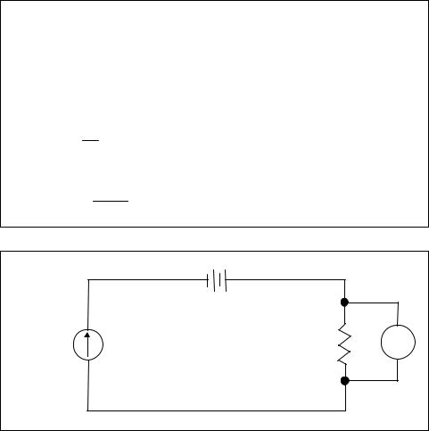
Voltage |
+ |
0 |
- |
a) Graph of AC Voltage
Time
b) Symbol for AC Voltage Source
Figure 3-3. Series resistance circuit
In this circuit, the current (I) flows from the negative terminal of the battery through the two resistors (R1 and R2) and back to the positive terminal. According to Ohm's law, the amount of current (I) flowing between two points in a circuit equals the potential difference (V) divided by the resistance (R) between these points. If V1 is the voltage drop across R1, V2 is defined as the voltage drop across R2, and the current (I) flows through both R1 and R2, then from Ohm's law we obtain the following:
V1 = IR1 and V2 = IR2
so that
Vt = IR1 + IR2
If we divided both sides of this equation by the current, I, in the series circuit, we obtain the following:
Vt/I = R1 + R2
Ohm’s law defines the total resistance of the series circuit as the total voltage applied divided by the current in the circuit or Rt = Vt/I. As a result, the total resistance of the circuit is given by the following equation:
Rt = R1 + R2
We can derive a more general equation for any number of resistors in series by using the classical law of conservation of energy. According to
76 Measurement and Control Basics
this law, the energy or power supplied to a series circuit must equal the power dissipated in the resistors in the circuit. Thus,
Pt = P1 + P2 + P3 ..... Pn
since power in a resistive circuit is given by P = I2R, we obtain the following:
I2Rt = I2R1 + I2R2 +I2R3 + ..... + I2Rn
If we divide this equation by I2, we obtain the series resistance formula for a circuit with n resistors:
Rt = R1 + R2 + R3 + ..... + Rn |
(3-10) |
Example 3-6 illustrates calculations for a typical series DC circuit.
Parallel Resistance Circuits
When two or more components are connected across a power source they form a parallel circuit. Each parallel path is called a branch, and each branch has its own current. In other words, parallel circuits have one common voltage across all the branches but individual currents in each branch. These characteristics contrast with series circuits, which have one common current but individual voltage drops.
Figure 3-4 shows a parallel resistance circuit with two resistors across a battery. You can find the total resistance (Rt) across the power supply by dividing the voltage across the parallel resistance by the total current into the two branches. In the circuit of Figure 3-4, total current is given by It = I1 + I2, where the current in branch 1 is given by I1 = Vt/R1 and the current in branch 2 is given by I2 = Vt/R2. Thus, It = Vt/R1 + Vt/R2. Since according to Ohm’s law total current is given by It = Vt/Rt, we obtain Equation 3-10 for total resistance, Rt, of two resistor in parallel:
1 |
= |
1 |
+ |
1 |
(3-11) |
|
R |
R |
R |
||||
|
|
|
||||
t |
|
1 |
|
2 |
|
Transforming this equation into a more useful form, we obtain the following:
|
R x R |
(3-12) |
|
R = |
1 |
2 |
|
t |
R + R |
|
|
|
1 |
2 |
|

Chapter 3 – Electrical and Electronic Fundamentals |
77 |
EXAMPLE 3-6
Problem: Assume that the battery voltage in the series circuit shown in Figure 3-3 is 6 Vdc and that resistor R1 = 1 kΩ and resistor R2 = 2kΩ , where k is 1,000 or 103. Find the total current flow (It) in the circuit and the voltage across R1 and R2.
Solution: To calculate the circuit current It, first find the total circuit resistance Rt using Equation 3-9:
Rt = R1 + R2
Rt = 1kΩ + 2kΩ
Rt = 3kΩ
Now, according to Ohm's law, we have:
It = Vt /Rt
It = 6V/3kΩ = 2 mA
The voltage across Rt (i.e., V1) is given by
V1 = R1It
V1 = (1kΩ )(2 mA) = 2V
Thus, the voltage across R2 (i.e., V2) is obtained as follows:
V2 |
= R2It |
|
|
|
|
|
V2 |
= (2kΩ |
) (2mA) = 4V |
|
|
|
|
|
_ |
It |
I1 |
_ |
I2 |
_ |
|
|
|||||
|
|
|
|
|
|
|
Vt |
+ |
|
R1 |
V1 |
R2 |
V2 |
|
|
|
+ |
|
+ |
|
|
|
|
|
|
Figure 3-4. Parallel resistance circuit

78 Measurement and Control Basics
We can derive the general reciprocal resistance formula for any number of resistors in parallel from the fact that the total current It is the sum of all of the branch currents, or
It = I1 + I2 + I3 + ..... + In
Since current flow is defined as I = dQ/dt, this is simply the law of electrical charge conservation:
dQt = dQ1 + dQ2 + dQ3 + . . . . .+ dQn dt dt dt dt dt
This law implies that, since no charge accumulates at any point in the circuit, the differential charge, dQ, from the power source in the differential time period, dt, must appear as charges dQ1, dQ2, dQ3 … dQn through the resistors R1, R2, R3 … Rn at the same time. Since the voltage across each branch is the applied voltage Vt and I = V/R, we obtain the following:
Vt |
= |
Vt |
+ |
Vt |
+ |
Vt |
+ . . . . . + |
Vt |
|
|
|
|
|
||||
Rt R1 R2 |
R3 |
|
Rn |
|||||
If we divide both sides of this equation by Vt, we obtain the total resistance of n resistors in parallel:
1 |
= |
1 |
+ |
1 |
+ |
1 |
+ . . . . . + |
1 |
(3-13) |
|
|
|
|
|
|||||
Rt |
R1 |
R2 |
R3 |
Rn |
|||||
To illustrate the basic concepts of parallel resistive circuits, let's look at Example 3-7.
Wheatstone Bridge Circuit
The Wheatstone bridge circuit, named for English physicist and inventor Sir Charles Wheatstone (1802-1875), was one of the first electrical instruments invented to accurately measure resistance. A typical Wheatstone bridge circuit is shown in Figure 3-5. The circuit has two parallel resistance branches with two series resistors in each branch and a galvanometer (G) connected across the branches. The galvanometer is a very sensitive elec- tric-current-measuring instrument that is connected across the bridge between points “a” and “b” when switch 2 is closed. If these points are at the same potential, the meter will not deflect. The purpose of the circuit is to balance the voltage drops across the two parallel branches to obtain zero volts across the meter and zero current through the meter. In the

Chapter 3 – Electrical and Electronic Fundamentals |
79 |
EXAMPLE 3-7
Problem: Assume that the voltage for the parallel circuit shown in Figure 3-4
is 12 V and we need to find the currents I |
, I |
, and I |
|
and the parallel resistance |
|||||
Rt, given that R1 = 30 kΩ and R2 = 30 kΩ t |
. 1 |
|
2 |
|
|||||
Solution: We can find the parallel circuit resistance Rt by using Equation |
|||||||||
3-12: |
|
|
|
|
|
|
|
|
|
|
|
R x R |
|
|
|
|
|
||
R = |
1 |
2 |
|
|
|
|
|
|
|
R + R |
|
|
|
|
|
||||
t |
|
|
|
|
|
||||
|
|
1 |
2 |
|
|
|
|
|
|
R = |
|
(30k)(30k) |
Ω = 15kΩ |
|
|
|
|
||
|
30k + 30k |
|
|
|
|
||||
t |
|
|
|
|
|
||||
The total current flow is given by the following equation:
I |
= |
Vt |
= |
12V |
= 0.8 mA |
|
15kΩ |
||||
t |
|
Rt |
|
|
|
|
|
|
|
|
The current branch 1 (I1) is obtained as follows:
I |
= |
Vt |
= |
12V |
= 0.4 mA |
|
30kΩ |
||||
1 |
|
R1 |
|
|
|
|
|
|
|
|
Since It = I1 + I2, the current flow in branch 2 is given by
I2 = It – I1 = 0.8 mA – 0.4 mA = 0.4 mA
S1 |
|
|
|
|
It |
R1 |
I1 I2 |
Rx |
|
_ |
|
|
|
|
Vt |
a |
G |
b |
|
+ |
||||
|
S2 |
IG |
||
|
R2 |
|
RS |
Figure 3-5. Wheatstone bridge circuit
80 Measurement and Control Basics
Wheatstone bridge, the unknown resistance Rx is balanced against a standard accurate resistor Rs to make possible precise measurement of resistance.
In the circuit shown in Figure 3-5, the switch S1 is closed to apply the voltage Vt to the four resistors in the bridge, and switch 2 is closed to connect the galvanometer (G) across the bridge. To balance the circuit, the value of Rx is varied until a zero reading is obtained on the meter with switch S2 closed.
A typical application of the Wheatstone bridge circuit is to replace the unknown resistor Rx with a resistance temperature device (RTD). An RTD is a device that varies its resistance in response to a change in temperature so the balancing resistor dial can be calibrated to read out a process temperature. In a typical application, an electronic device that is designed to convert resistance into temperature is connected to the bridge circuit to measure and display the temperature directly.
When the bridge circuit is balanced (i.e., there is no current through galvanometer G), the bridge circuit can be analyzed as two series resistance strings in parallel. The equal voltage ratios in the two branches of the Wheatstone bridge can be stated as follows:
I2 Rx |
= |
I1 R1 |
(3-14) |
|
|
||
I2 Rs I1 R2 |
|
||
Note that I1 and I2 can be canceled out in the previous equation, so we can invert Rs to the right side of the equation to find Rx as follows:
R = R |
R1 |
(3-15) |
|
||
x s R |
|
|
|
2 |
|
To illustrate the use of a Wheatstone bridge, let's consider Example 3-8.
Instrumentation Current Loop
The brief discussion on resistive circuits earlier in this chapter served as a starting-off point for this section on instrumentation current loops. The dc current loop shown in Figure 3-6 is used extensively in the instrumentation field to transmit process variables to indicators and controllers. It is also used to send control signals to field devices to manipulate process variables such as temperature, level, and flow. The standard current range used in these loops is 4 to 20 mA, and this value is normally converted to 1 to 5 V dc by a 250 Ω resistor at the input to controllers and indicators.
Chapter 3 – Electrical and Electronic Fundamentals |
81 |
EXAMPLE 3-8
Problem: Assume a Wheatstone bridge with R1 = 1 kΩ and R2 = 10kΩ . If Rs is adjusted to read 50Ω when the bridge is balanced (i.e., the galvanometer reading is at zero), calculate the value of Rx.
Solution: We can use Equation 3-15 to determine Rx:
Rx = Rs R1
R2
Rx = 50Ω 1KΩ = 5Ω 10KΩ
_ |
+ |
|
|
|
24V dc |
|
+ |
|
|
|
|
|
|
|
||
4 to 20 ma |
Temperature |
|
Ω |
|
|
|
Current |
250 |
R |
TI |
|||
Transducer |
||||||
Transmitter |
|
|
_ |
|
||
|
|
|
|
|||
|
|
|
|
|
Figure 3-6. Typical 4-to-20 mA current loop
These instruments are normally high-input-impedance (Zin > 10 MΩ ) electronic devices that draw virtually no current from the instrument loop.
There are two main advantages to using the 4-to-20 mA current loop. First, only two wires are required for each remotely mounted field transmitter, so a cost savings is realized on both labor and wire when installing field devices. The second advantage is that the current loop is not affected by electrical noise or changes in lead wire resistance caused by temperature changes.
Selecting Wire Size
You must consider several factors when selecting the wire size for a control application. One factor is the permissible power loss (P = I2R) in the electrical line. This power loss is electrical energy being converted into

82 Measurement and Control Basics
heat. If the heat produced is excessive, the conductors or system components may be damaged. The use of large-diameter (low-wire-gauge) conductors will reduce the circuit resistance and, therefore, the power loss.
However, larger-diameter conductors are more expensive than smaller ones and they are more costly to install, so you will need to make design calculations to select the proper wire size.
A second factor when selecting wire is the resistance of the wires in the circuit. For example, let's assume that we are sending a full-range 20 mA dc signal from a field instrument to a programmable controller input module that is located 2,000 feet away, as shown in Figure 3-7.
|
Rw |
|
|
|
4 to 20 ma |
_ |
+ |
|
|
|
|
|
||
|
24V dc |
+ |
|
+ |
|
|
|
PLC |
|
|
|
|
|
|
Field |
|
250 Ω |
R |
Analog |
Instrument |
|
_ |
|
Input |
|
|
|
_ |
|
|
|
|
|
|
|
Rw |
|
|
|
|
2000 ft |
|
|
|
Figure 3-7. Voltage drop in instrument loop
Assuming that we are using 20 AWG wire, we can easily calculate the wire resistance (Rw). Using data from Table 3-2, we see that 20 AWG wire has a resistance of 10.4Ω per 1,000 ft at 25°C. So the resistance for the 4,000 feet of wire is calculated as follows:
Rw = (10.4Ω /1000 ft)(4000 ft) = 41.6Ω
This resistance increases the load on the 24 Vdc power supply that is used to drive the current loop. You can calculate the voltage drop Vw in the wire when the field instrument is sending 20 ma of current to the programmable controller analog input module by using Ohm's law:
Vw = IRw = (20 mA)(41.6Ω ) = 0.832 Volts
A third factor when selecting wire is the current-carrying capacity of the conductor. When current flows in a wire, heat is generated. The tempera-
Chapter 3 – Electrical and Electronic Fundamentals |
83 |
ture of the wire will rise until the heat that is radiated away, or otherwise dissipated, is equal to the heat generated in the conductor. If the conductor is insulated, the heat produced is not dissipated so quickly as it would if the conductor were not insulated. So, to protect the insulation from excessive heat, you must keep the current flowing in the wire below a certain value. Rubber insulation will start to deteriorate at relatively low temperatures. Teflon™ and certain plastic insulations retain their insulating properties at higher temperatures, and insulations such as asbestos are effective at still higher temperatures.
You could install electrical cables in locations where the ambient temperature is relatively high. In these cases, the heat produced by external sources adds to the total heating of the electrical conductor. When designing a control system you must therefore make allowances for the ambient heat sources encountered in industrial environ-ments. The maximum allowable operating temperature for insulated wires and cables is specified in manufacturers' electrical design tables.
Table 3-3 gives an example of the maximum allowable current-carrying capacities of copper conductor with three different types of insulation. The current ratings listed in the table are those permitted by the National Electrical Code. This table can be used to determine the safe and proper wire size for any electrical wiring application. Example 3-9 will help to illustrate a typical wiresizing calculation.
Table 3-3. Ampacities of Insulated Copper Conductor National Electrical Code
|
|
75°C (167°F) Types: |
|
|
Conductor |
60°C (140°F) |
FEPW, RH, RHW, |
85°C (185°F) Type: V18 |
|
Size (AWG) |
Types: TW, UF |
THHW, THW, THWN, |
||
|
||||
|
|
XHHW, USE, ZW |
|
|
|
|
|
|
|
14 |
20 |
20 |
25 |
|
12 |
25 |
25 |
30 |
|
10 |
30 |
35 |
40 |
|
8 |
40 |
50 |
55 |
|
6 |
55 |
65 |
70 |
|
|
|
|
|
Power Supplies
It is important for process control users to have a basic understanding of the design and operation of dc power supplies because of their wide use in control systems applications. DC power supplies use either half-wave or full-wave rectification, depending on the power supply application in question. Figure 3-9 shows the output waveforms produced by half-wave

84 Measurement and Control Basics
EXAMPLE 3-9
Problem: Calculate the proper wire size for the 120 Vac feed to the programmable controller system shown in Figure 3-8, assuming a maximum ambient temperature of 60°C.
Solution: The total ac feed current is the sum of all the branch currents, or
It = I1 + I2 + I3 + I4
It = 8 A + 2 A + 5 A + 5 A
It = 20 A
Using Table 3-3, we can see that the main power conductors (hot, neutral, and ground) must have a minimum size of 14 AWG.
L1 |
L2 |
|
120 Vac |
I1 = 8A |
Main PLC |
|
Rack 0 |
I2 = 2A |
Remote PLC I/O |
|
Rack 1 |
I3 = 5A |
Remote PLC I/O |
|
|
|
Rack 2 |
I4 = 5A |
Remote PLC I/O |
|
|
|
Rack 3 |
Figure 3-8. PLC wire-sizing application
and full-wave rectification. A schematic diagram of a half-wave rectifier is shown in Figure 3-10. In the circuit in Figure 3-10, the positive and negative cycles of the ac voltage across the secondary winding are in phase with the signal at the primary. This is indicated by the dots on each side of the transformer symbol.