

Diss / 4
.pdfIEEE TRANSACTIONS ON SIGNAL PROCESSING, VOL. 58, NO. 7, JULY 2010 |
3647 |
Detection–Estimation of Very Close Emitters:
Performance Breakdown, Ambiguity, and General
Statistical Analysis of Maximum-Likelihood
Estimation
Yuri I. Abramovich, Fellow, IEEE, and Ben A. Johnson, Senior Member, IEEE
Abstract—We reexamine the well-known problem of “threshold behavior” or “performance breakdown” in the detection-estima- tion of very closely spaced emitters. In this extreme regime, we analyze the performance for maximum-likelihood estimation (MLE) of directions-of-arrival (DOA) for two close Gaussian sources over the range of sample volumes and signal-to-noise ratios (SNRs) where the correct number of sources is reliably estimated by informationtheoretic criteria (ITC), but where one of the DOA estimates is severely erroneous (“outlier”). We show that random matrix theory (RMT) applied to the evaluation of theoretical MLE performance gives a relatively simple and accurate analytical description of the threshold behavior of MLE and ITC. In particular, the introduced “single-cluster” criterion provides accurate “ambiguity bounds” for the outliers.
Index Terms—Direction-of-arrival (DOA) estimation, max- imum-likelihood estimation, random matrix theory, signal detection, signal resolution.
I. INTRODUCTION AND BACKGROUND
UNDAMENTAL limitations on the ability to estimate F the number of sources 

 impinging upon an
  -sensor antenna array and to estimate their DOAs (so-called “threshold behavior” [1]–[5]) remains an important and still frequently addressed signal processing problem [6]–[10]. The threshold behavior of an MLE algorithm occurs as signal-to-noise ratio (SNR)

 and/or sample volume

 drop below some threshold value, and manifests as having the observed estimation accuracy rapidly depart from Cramér–Rao bound (CRB) predictions [7]–[11]. While this phenomenon has long been described in the literature, MLE threshold behavior remains largely unknown, except for some simple scenarios. According
Manuscript received February 15, 2009; accepted February 04, 2010. Date of publication April 01, 2010; date of current version June 16, 2010. The associate editor coordinating the review of this paper and approving it for publication was Dr. Brian Sadler. This work was supported in part by DSTO/LMA R&D Collaborative Agreement 290905.
Y. I. Abramovich is with the Intelligence, Surveillance, and Reconnaissance Division, Defence Science and Technology Organization (DSTO), Edinburgh SA 5111, Australia (e-mail: yuri.abramovich@dsto.defence.gov.au).
B. A. Johnson is with Lockheed Martin Australia and the Institute for Telecommunications Research, University of South Australia, Mawson Lakes SA 5095, Australia (e-mail: ben.a.johnson@ieee.org).
Color versions of one or more of the figures in this paper are available online at http://ieeexplore.ieee.org.
Digital Object Identifier 10.1109/TSP.2010.2047334
to Forster [12], “no general non-asymptotic results are available for the performance evaluation of the MLE method, and each problem requires a special investigation.” For this reason, most published results have been derived for the DOA estimation of a single source impinging on an antenna array, or equivalently, for a single complex frequency estimation from a finite number of discrete time observations [11]–[16]. Here, MLE has a simple practical implementation, and so any theoretical derivations can be directly tested by Monte-Carlo simulations. For multiple sources, the threshold behavior has been analyzed primarily with the aid of Barankin bounds [17]–[19], while simulations have been conducted for scenarios that could still be addressed by a 1-D maximum-likelihood (ML) search. In [17], for example, the authors assumed the parameters of one of the two sources are known a priori, which obviously alters the original detection-estimation problem; 2-D search results were reported only recently [7].
Because of computational problems associated with exhaustive search for the global maximum of the multi-extremal non-convex likelihood function, assessment of threshold MLE behavior for multiple sources has been often based on indirect or MLE-proxy (MLE approximation) methodologies. This approach was used in [20], where the authors examined the threshold behavior in detection-estimation of two closely-spaced independent equi-power Gaussian sources in noise. In particular, the authors of [20] established that the “detection SNR threshold” for closely spaced sources is significantly smaller than the “MLE SNR threshold.” Those authors defined the “detection SNR threshold” as the minimum SNR for a given scenario 


 such that a selected information-theoretic criterion (ITC) (in this case MDL), provides detection of the correct number of sources (

 in this case) with sufficiently high probability (say,


 ). Obviously, an ITC-based detection algorithm is directly implementable, and therefore verification of the analytical predictions for this “detection SNR” threshold


 by Monte-Carlo simulations were conducted in [20] with no difficulties.
On the other hand, for the MLE SNR threshold, no direct MLE simulations were reported in [20] to support the analytical findings. Instead the authors specified this MLE SNR threshold as the SNR value 


 such that
(1)
1053-587X/$26.00 © 2010 IEEE
3648 |
IEEE TRANSACTIONS ON SIGNAL PROCESSING, VOL. 58, NO. 7, JULY 2010 |
where the true DOAs are 


 , while
 and
and 
 are the CRBs of the standard deviations of the DOA estimates


 . Since then, this criterion has been frequently used by scientific community as defining the “ultimate resolution limit” [21]. Yet, poor accuracy of CRB predictions within the threshold area is well established by analysis of the single source (tone) detection estimation in noise [11], [14], [15] which means that MLE may actually “break” at a larger SNR than this CRB-based resolution limit. Rather than experimentally validating the criterion using MLE, Lee and Li instead cited the famous Kaveh–Barabel formula for the MUSIC SNR threshold [22], implying that the validation of the MLE SNR threshold could be performed by MUSIC simulations.
It is now well-known that MUSIC “breaks down” at SNR threshold values that significantly exceed the genuine MLE SNR threshold [23], and other MLE-proxy DOA estimation algorithms that perform better than MUSIC have been introduced [24]–[26], but since MLE-proxy DOA estimation techniques are approximations which do not guarantee the global likelihood extremum, their behavior cannot be directly associated with the genuine MLE threshold phenomenon. It is impossible to exclude that we are dealing with proxy-specific behavior (as per MUSIC “breakdown”) and not with the intrinsic limitations of MLE.
Still, the earlier results of Lee and Li [20] and our own observations [24] indicate the existence of a very important MLE phenomenon. Indeed, the assertion made in [20] that as 


 , the ratio


 “grows without bound” implies that within quite a broad range of closely spaced multiple source scenarios, MLE-based detection-estimation unavoidably produces a severely erroneous result.
Let us clearly state that the fact that any statistical technique, including MLE, “breaks” at some point with insufficient training sample support or/and SNR is well expected and trivial. What is less trivial and more dangerous is that detection “breaks” at significantly smaller SNR threshold values than estimation does. The “bright side” of this story, broadly used so far, allows the number of sources to be properly estimated when analyzing DOA estimation accuracy of different ML-proxy routines such as MUSIC. The “dark side” of this story is that by advancing our DOA estimation techniques towards the genuine MLE limit, we inevitably approach the area where with high probability we detect the correct number of sources, but with same high probability, at least one of  DOA estimates will be severely erroneous. Therefore, it seems quite important to specify more accurately the actual MLE performance in the threshold area.
Apart from the above-mentioned approaches used in [20], we can refer to two other techniques used for MLE performance analysis in the threshold region. First there is the “large error” Barankin bound (BB) analysis, which in most cases is not directly computable, with numerous attempts to find computable BB approximations (e.g., see list of references in [19]). The second approach stems from Rife and Boorstyn [13] who derived the theoretical MLE variance for a single tone under the assumption that when a single tone (or DOA) estimate is within the beampattern lobe, its probability distribution is Gaussian with variance given by the CRB, and otherwise, it is uniformly
distributed within 


 . Their approach has been variously modified [6], [12] for multiple sources, by using properties of deterministic SNR-asymptotic
  SNR
SNR 

 or sample sup- port-asymptotic


 functions. For threshold conditions with very limited SNR and
  , these techniques are not particularly well justified and are much more complicated for multiple sources than for a single tone.
In this paper, we therefore strive to more directly describe the actual behavior of MLE in the threshold area. As a result, the organization of this paper is somewhat unusual. Since it is not evident what analytic tools are sufficiently accurate in this threshold regime, we start in Section II from a detailed analysis of Monte-Carlo simulations in order to clarify MLE breakdown behavior. Unlike most of the above referenced studies, we rely on the exhaustive search for the global likelihood maximum, in order to explore the genuine MLE properties. Naturally, we have to consider a relatively small number  of sources in order to keep the complexity of
  -dimensional exhaustive search manageable. For this reason, we confine this analysis to the minimal number of closely separated sources

 . We start with the same three-sensor


 two-source scenario as Lee and Li in [20], so that we can compare our and [20] results in identical conditions, but since such a small antenna dimension leaves quite legitimate concerns whether this scenario is sufficiently representative, we then consider a scenario with an
 -element uniform linear antenna (ULA) and
sources in order to demonstrate the generic nature of the established MLE properties in the threshold region. The examination of the Monte-Carlo simulations provides insights into the “mechanism” of MLE breakdown, that in turn allow us to propose the use of Random Matrix Theory (RMT) [27] (a.k.a. General Statistical Analysis, GSA) [28] methodology for analytical description of MLE threshold behavior. (Section III). Sufficiently high accuracy of these predictions is demonstrated in Section IV. Section V summarizes and concludes this paper.
II.MLE PERFORMANCE BREAKDOWN: SIMULATION RESULTS
A. Motivations and Model Selection
We start the main body of this paper with simulations using the (impractical) two-dimensional search for the global likelihood maximum, motivated by three major issues.
•The anticipated inaccuracy of conventional asymptotic


 MLE analysis (in particular, the CRB) in the “threshold region.”
•The significant difference in the “performance breakdown” conditions in MUSIC (referred to by Lee and Li in [20]), and much better threshold performance of more advanced “MLE-proxy” routines in [24].
•Our inability to claim the global optimality of the de-
tection-estimation solutions delivered by this advanced “MLE-proxy” routine in [24], leaving some doubt as to the properties of genuine MLE.
We first consider the scenario of Lee and Li [20]: a 

 element array uniformly spaced at half-wavelength spacing,
with 

 independent Gaussian emitters located at


 , with equal power


 , and a unity white noise

ABRAMOVICH AND JOHNSON: DETECTION–ESTIMATION OF VERY CLOSE EMITTERS |
3649 |
floor 


 . We simulate
  independent identically distributed (iid) training data samples
(2)
where 


 is the
  -variate complex (circular) Gaussian pdf with zero mean and positive-definite covariance matrix
  . For input data that is a mixture of
  independent plane-wave signals in white noise, we have
|
(3) |
where the source powers in |
are all pos- |
itive, and |
is the matrix of |
antenna array manifold (steering) vectors  for the DOAs (azimuthal angle)
 .
.
In this paper, in addition to the traditional ITC-based detection followed by MLE [29], we consider a joint detection-esti- mation approach that involves direct thresholding of the globally maximized LR values, with some similarity to the gener- alized-likelihood ratio test (GLRT) [30]. We do so not because this GLRT-based algorithm outperforms ITC (in fact, we have previously demonstrated that its detection performance is similar [31], [32]), but because examination of the distribution of the likelihood ratio for both the proper and incorrect number of
sources provides useful insights. |
|
|
|
Let |
be the hypothesized number of sources, then the EL |
||
method is to estimate the set of |
parameters |
|
|
|
|
|
(4) |
if the white-noise power is known, or the set of |
param- |
||
eters |
otherwise. We consider a “conventional |
||
number” of identifiable sources |
, and for the arbitrary |
||
antenna array geometry identifiability is an additional restriction, as usual.
The totality of estimates |
or |
uniquely describes |
a covariance matrix model, |
or |
say, and in the |
MLE paradigm, the optimal estimates are those that yield the global maximum to the likelihood function (LF)
|
|
(5) |
|
where the sample covariance matrix is |
|||
. Instead |
|||
of this specific LF, we may use any other function that is a product of the LF and a nonzero number that does not depend on  or
or 
 [33]. In particular, the likelihood ratio
LR

(6)
may be used as the LF when 

 where we just multiplied (5) on


 . The crucial advantage of using the LR LR

 instead of the LF


 , and in general the
stochastic (unconditional) model (2)–(5) rather than the deterministic (conditional) one [29] for the practical ML-proxy algorithms introduced in [24] is that the pdf of LR

 is not a function of
  . Indeed,
LR |
|
(7) |
|
||
where |
, i.e., is a random matrix with |
|
a complex Wishart distribution, with all parameters known a priori. This, together with the fact that LR


 LR
LR

 , means that we can derive or precalculate any desired false-alarm
threshold |
for LR |
that with a given (high) probability |
|
must be exceeded by LR |
, and hence by LR |
. In terms |
|
of the global likelihood search, it is of course important to note that the search for the maximum of LR

 is identical to that of the LF


 .
.
To complete the problem description, the respective detection estimates  for GLRT-based detection-estimation and ITC are
LR |
|
LR |
(8) |
where the factor  depends on the precise method (AIC, MDL, MAP, etc.) [34]. In (8), for every
  , the likelihood ratio should be (globally) maximized over the set of parameters
  that specify
  , while the smallest
  in LR
in LR

 exceeding the threshold, is treated as the estimated number of sources
  with ML estimates

 .
.
B. Simulation Results (Lee and Li [20]), 


We begin the presentation of our results with a CRB analysis of the three-sensor scenario with two equi-power sources
at |
and |
training samples (“snap- |
shots”). |
|
|
For the |
CRB based “resolution |
limit” |
|
, we achieve a CRB equal to half the source sep- |
|
aration at an SNR of 37 dB (i.e., |
dB). In order to |
|
specify the ITC “detection SNR threshold,” we conducted 

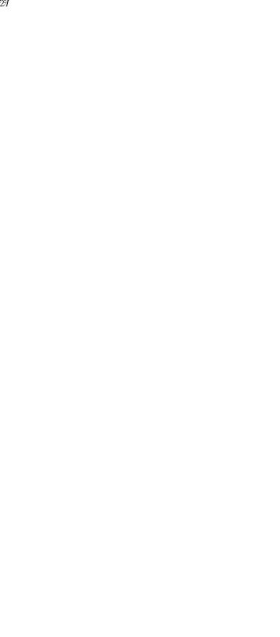
 Monte-Carlo simulations per datum, as illustrated by Fig. 1. This experiment revealed a
 % probability of MDL failure (underestimation of the number of sources) at about 22 dB. For the asymptotically more accurate MAP criterion, the same failure occurs at about 24 dB. The AIC method is well known for its tendency to overestimate, and here the half-failure rate is at approximately 19 dB. This is consistent with [20], which specified that
 dB
dB 


 SNR
SNR 


 dB. Fig. 1 also presents a sample cumulative distribution of MUSIC failure probability for the same scenario. This failure can occur in one of two ways for this small array scenario: either the entire MUSIC pseudo-spectrum has only one peak, or MUSIC is unable to successfully resolve the two close sources and produces an “outlier” (by selecting an erroneous spurious peak). As usual, we define a DOA estimate to be an outlier if it is more than half of the source separation from the nearest true DOA, i.e., the MUSIC trials are valid here if


 and
and 


 . As the SNR decreases, we see that MUSIC begins to become unreliable at SNRs far greater than
3650 |
IEEE TRANSACTIONS ON SIGNAL PROCESSING, VOL. 58, NO. 7, JULY 2010 |
Fig. 1. ITC and MUSIC breakdown for simulated scenario.
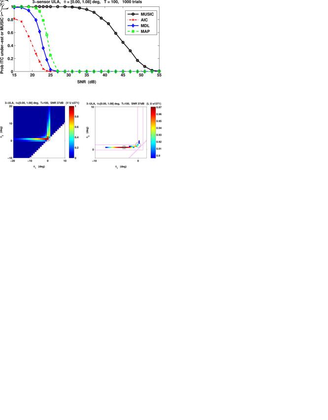
Fig. 2. Example full LR for (left) a successful ML DOA estimation, and thresholded LR (right) an unsuccessful trial (where an outlier is generated), arbitrary-power model. For the unsuccessful trial, 
dB, LR . The circle marks the exact DOAs, the square shows the discretized maximum, and the diamond is the location of the optimized maximum.
the CRB “resolution limit” (


 dB), or even at the Kaveh–Barabel prediction of 40 dB; indeed at 40 dB, MUSIC is almost completely “broken” (80% failure rate).
As expected, MUSIC performance fails to mirror genuine MLE behavior in this threshold region. However, as discussed, the results of the CRB predictions are also expected to be inaccurate in this threshold region. Therefore our first task is to investigate the actual MLE behavior by simulation in the SNR range 


 (22–37 dB for the Lee and Li scenario). Along with proper solutions, we expect a continuum of completely erroneous solutions to appear that are “as likely” or “more likely” than the true covariance matrix. We term this phenomenon statistical nonidentifiability or ambiguity [35], [36].
To explore the actual performance of global ML DOA estimation, we conducted a direct exhaustive search for the global maximum of the function LR

 (5) over a discretized 2-D grid (with


 ), similar to [7]. First, at every point


we computed the corresponding power estimates as [29]
(9)
for
(10)
for 
Because the grid was sufficiently fine, further gradient-type optimization did not materially modify the results, although we did this additional final optimization throughout the paper just to ensure strict MLE optimality of the solution.
We emphasize that the global search and in fact, the way we assign each DOA estimate to either 
 or
or 
 , is performed in the natural order


 . This means that the smallest DOA estimate within the range


 is always treated as the estimate of
 , while the estimate
 is treated as the estimate of


 in our scenario. This pragmatic rule means that in some cases,
 may be actually closer to
 than to
 , but in this case, the second estimate


 is even further away from
 than
than 
 . In this study we have used the normalized form (6) of the likelihood function, which is the likelihood ratio. For each trial, we have calculated the LR value for the actual covariance matrix LR

 , and compared it with the likelihood ratio of the MLE solution
 , where
|
(11) |
and |
are the generated ML estimates of the th source |
parameters. |
|
Since the pdf for LR

 does not depend on
  as illustrated by (7), we calculated this scenario-invariant pdf offline to a high level of fidelity by using ten million Monte-Carlo trials. This allows us to readily assign thresholds corresponding to different
levels of false alarm probability. Using |
|
, we found |
|
that corresponding false alarm threshold is |
. This |
||
means that with probability |
LR |
and therefore |
|
LR |
should exceed the LR value |
|
. |
We begin our analysis at the SNR of 37 dB, which is the “CRB resolution limit.” Two example Monte-Carlo trials that illustrate our search for the global likelihood maximum appear at Fig. 2. The first subfigure shows the typical shape of the LR function; away from the two perpendicular “arms” that are centered at 


 , the likelihood ratio is vanishingly small. In this particular random trial, the final DOA estimate is very accurate:


 dB. The second subfigure shows the LR (for clarity, only where it exceeds the threshold
 ) for a different, less successful random trial.
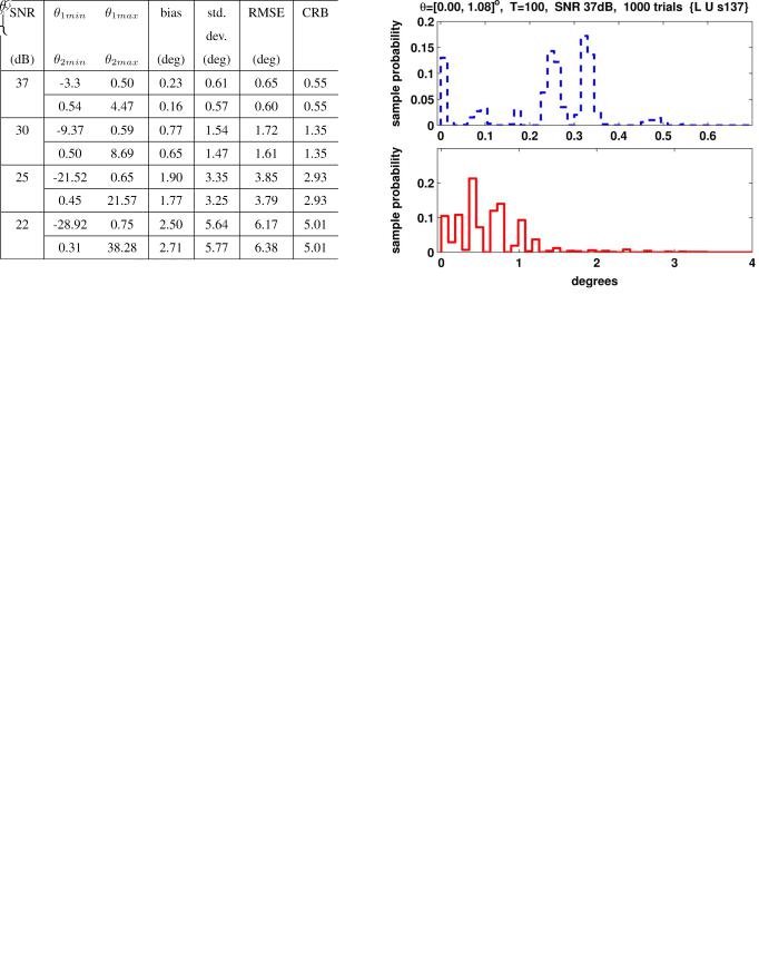
In this second example trial, the maximum of the LF (6) is very far from the true DOAs, well above the CRB prediction. In Table I we provide a statistical description of Monte-Carlo simulation results, with 1000 trials per datum for this scenario and different SNRs (37, 30, 25, and 22 dB). For each SNR value,
the estimates |
and |
are bounded by the sample support |
intervals |
|
|
|
|
(12) |
where 


 and
and 


 are the minimum and the maximum values of the estimates

 observed over the 1000 trials; and described by bias, standard deviation and total RMSE of

 , and the CRB,


 . Analysis of these results leads to a number of important observations.
While observed RMSE and standard deviation values are not that different from the CRB predictions, the sample support intervals in Table I clearly indicate a significant departure of the errors pdf from the conventional Gaussian one. Detailed analysis of the experimental data reveals that} for the 


 37-dB SNR, we still observe a small number of solutions where both
ABRAMOVICH AND JOHNSON: DETECTION–ESTIMATION OF VERY CLOSE EMITTERS |
3651 |
TABLE I


ML DOA estimates 

 and
and 

 are reasonably accurate, as per the example shown in the first subfigure in Fig. 2, but the majority of the results for SNR

 dB, and practically all results for the smaller SNRs, have only one accurate DOA estimate,

 or
or 

 with the other one being significantly less accurate. In fact, the actual behavior of MLE within this interval
 dB
dB  SNR
SNR 

 dB, is well described by the event
(13)
where  and
and  are Bernoulli random numbers of value either zero or one. The estimate
 is the “good” estimate, located in vicinity of the midpoint between the two sources. The estimate
 is an outlier distributed over the “MLE ambiguity region”
|
|
(14) |
where |
is the “extreme” outlier registered over the Monte- |
|
Carlo trials. |
|
|
For |
, the |
and in |
|
|
(15) |
are similarly defined.
For SNR 


 dB, the probability of getting two “good” DOA estimates (as in the first subfigure of Fig. 2) is still significant, but for the smaller SNR we observe that

 , meaning that both estimates

 and
and 

 are practically never simultaneously “good.” This observation is supported by Fig. 3, where we introduce sample pdfs for the error in the “best” of the two estimates


(16)
and the worst of these two ML DOA estimates
(17)
for the scenario with SNR 

 dB.
dB.
First of all, we can see that the “best” estimate error hardly reaches the value of 0.5 , while the CRB prediction for stan-
Fig. 3. Sample pdf of (upper)  0
0 
 0
0  , (lower)
  0
0

 0
0  .
.
dard deviation is 0.57 in this case. At the same time, the second, “worst” estimate of the two

 and
and 

 spreads to


 , far beyond the CRB prediction.
In fact, the described behavior has quite a simple physical interpretation. Indeed, when approaching the threshold condition (SNR 

 dB;
dB; 


 , in our case), the MLE algorithm starts to lose its ability to resolve the close sources and instead produces an estimate of a single source, close to the “center of gravity” of the two sources. For equi-power sources, this “center of gravity” is obviously in the midpoint


 between the two DOAs. The second DOA estimate is an outlier distributed over the MLE ambiguity region


 that depends on SNR and sample support
  for the given scenario
and |
. |
|
|
|
Interestingly enough, since practically half of estimates |
|
|||
(SNR |
dB) are “good” (i.e., |
), while the rest of |
||
them are “bad” |
), the overall RMSE for the |
is |
||
not dramatically different from the CRB prediction, especially for the high SNR of 37 dB. Obviously, the same is true for the
estimate |
. |
In Fig. 4, we introduce our sample pdfs for the estimates |
|
and |
for SNR 37, 30, 25, and 22 dB complementing the |
data introduced in Table I. Each of these pdfs may be treated as the convolution of pdfs for the “good” 
 and “bad” estimates
 in (13), illustrated in turn, by Fig. 3. These pdfs in Fig. 4 demonstrate that as the SNR is reduced within our “SNR ambiguity range”


 SNR
SNR 


 , the “MLE ambi-
guity region” expands, eventually reaching 37 at SNR |
dB. |
|||
Moreover, the pdfs for |
and |
start to overlap, which was |
||
not the case at SNR |
dB, meaning we frequently observe |
|||
estimates |
or |
. |
|
|
Recall that for single tone threshold, Rife and Boorstyn in [13] described the ML estimate being “good” (described by the CRB) with a certain probability and “bad” (an outlier) with the complementary probability. We suggest that for the two source case, this “bad” description may be modified to state that while we always get two ML estimates, one of them is “good” and
3652 IEEE TRANSACTIONS ON SIGNAL PROCESSING, VOL. 58, NO. 7, JULY 2010
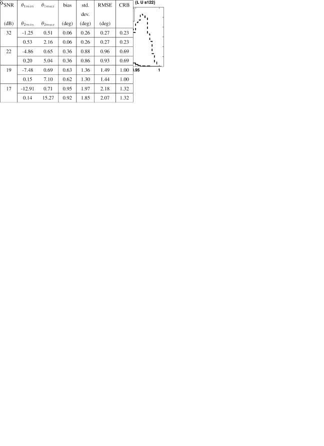
TABLE II


Fig. 4. Statistical analysis of MLE results for the arbitrary-power model.
Fig. 5. Statistical analysis of MLE results at 22 dB SNR.
described by the CRB for the single source at the midpoint  and power


 , while the other is an outlier, distributed over the “MLE ambiguity region.”
Finally, further examination of our simulation results can be used to demonstrate how SNR reduction makes the single source model more and more “likely,” eventually leading to a singlesource model acceptable to our GLRT-based detection-estima- tion rule (8). To illustrate, in Fig. 5, we show sample pdfs of the LR for both the true two-source scenario with 
 and
and 
 and the “midpoint” model with


 for SNR

 dB; the equivalent plots for 25, 30, and 35 dB are not shown.
The maximum LR (over 1000 trials) of the single-source model for SNR 

 dB reached LR


 ; for SNR

 dB, it reached LR


 , and finally, for SNR

 dB, illustrated by Fig. 5, the maximum reached LR


 , which is far above the LR threshold


 in (8), calculated for


and 


 . This indicates that at this low SNR, there is finally a substantial probability that LR

 will exceed the
 threshold and therefore, the GLRT-based detection-estimation rule (8) will treat our data as being described by a single source covariance matrix. This probability is consistent with the ITC probability of underestimation


 illustrated by Fig. 1 for 22 dB.
C. Simulation Results for 


The reader will note that Lee and Li’s small array scenario leaves legitimate concerns regarding validity of our conclusions for larger array dimensions 


 and smaller sample support


 . We have therefore considered the two source equi-power scenarios in a larger eight-sensor uniform linear antenna array, with considerably lower sample support and a similar source spacing (


 The scenario reaches the “CRB resolution limit”


 at SNR

 dB. On the other hand, at SNR

 dB the probability of underestimation of the correct number of sources


 by the MAP ITC criterion is equal to 0.2, and at SNR

 dB it is equal to 0.95. Therefore, the “SNR ambiguity range” here is quite small, roughly


 dB
dB
 SNR
SNR 


 dB
dB . In the simulations, we also expand our examined SNR range up
to 32 dB to include values |
. |
|
For SNR |
dB, results of 1000 Monte-Carlo trials is rep- |
|
resented by data in Table II. One can see that for SNR 

 dB where the


 , the ML DOA estimates still diverge from the CRB quite substantially. While the actual


 only marginally exceeds the CRB, the support interval
(18)
and the actual pdf (similar to that in Fig. 4, but not introduced here) make it clear that divergence from the Gaussian pdf is quite significant. Indeed, a Gaussian pdf with standard deviation of 


 would significantly underestimate the actual probability of occurrence of large errors (

 , say) that were frequently observed in these simulations. It is important to note that even for the other extreme when SNR
 , the actual pdf of the DOA estimate is also proven in [37] to divert from Gaussian for a finite (small) sample support
  . Now we observe that in the threshold area this departure is even more profound.
As with the earlier scenario, for lower SNR values within the “SNR ambiguity range,” we observe the now familiar trend of the growing “MLE ambiguity range” 


 with decreasing SNR (Table II).
D. Main Simulation Observations
One can see that in both analyzed scenarios, we observe the same MLE “breakdown phenomenon.” Specifically, for closely separated sources, at SNR values well above the “CRB resolution threshold” 


 , the actual MLE errors depart from traditional asymptotic


 description via a multivariate Gaussian pdf with the Fisher Information Matrix (FIM) inverse as the covariance matrix. The actual MLE errors reach significantly larger values than provided by a Gaussian pdf with the standard deviation predicted by the CRB. At SNRs that are close to the “CRB resolution threshold”


 , MLE loses its capability to resolve the two close sources, and generates one DOA estimate that is always located close to the “center of gravity” of the two sources, while the second outlier DOA
ABRAMOVICH AND JOHNSON: DETECTION–ESTIMATION OF VERY CLOSE EMITTERS |
3653 |
estimate fluctuates within the “MLE ambiguity region” that depends on SNR and sample support. The “MLE ambiguity region” becomes larger and eventually, at sufficiently small SNR, the power estimate of the outlier becomes so small that the covariance matrix model with a single “midpoint” source may exceed the likelihood ratio threshold 
 in our GLRT-based detection-estimation routine (5). In our simulations, this SNR value quite accurately coincides with the ITC SNR threshold


 , below which a single source is detected.
This experimental analysis of the genuine MLE performance has supported the Lee and Li conclusion that within the SNR ambiguity range (


 SNR
SNR 


 , detection-estimation will fail, with one of the DOA estimates being an outlier. We also observed that the “MLE ambiguity region” extends far beyond the SNR range indicated by the use of the CRB standard deviation. Therefore, an analytical prediction of the “MLE ambiguity region”


 that augments the error standard deviation prediction by the CRB would be useful and motivates the next section.
III. G-ASYMPTOTIC ANALYSIS OF MLE PERFORMANCE
IN THE THRESHOLD REGION
A. Statistical Ambiguity as Random Matrix Similarity Test
As discussed, our goal is to provide an analytical description to the “MLE ambiguity region,” which was introduced as a MLE confidence interval based on Monte-Carlo simulations: 


 . In order to justify our approach to
derivation of the bounds ( |
, |
), let us reconsider the MLE |
problem, as it is formulated by (6) |
|
|
|
|
(19) |
where |
is the covariance matrix model uniquely recon- |
|
structed using the set of parameters . For |
(for the true |
|
number of sources), we obviously have LR |
LR , |
|
where  is the true covariance matrix of the input data. Recall that the likelihood ratio (6) is the optimum one to test the hy-
pothesis [38] |
versus the al- |
ternative |
given . Therefore, |
maximization of the likelihood function (ratio) may be treated as finding the best “whitening” transformation (matrix 


 ) within a given class of restricted models for
  . In DOA estimation problem, this class is limited by representation (3) for a number of uncorrelated plane-wave sources in noise. For the
true covariance matrix |
|
|
when |
|
||||
|
|
|
|
|
|
|
|
(20) |
|
|
|
|
|
|
|
|
|
the pdf of the LR |
is known a priori even when the covari- |
|||||||
ance matrix is not, since it does not depend on |
and is fully |
|||||||
specified by parameters |
and |
|
|
(see (7)). |
|
|||
Conceptually |
at least, |
for |
|
|
any |
and |
||
|
|
|
|
, |
we may attempt |
to find a |
||
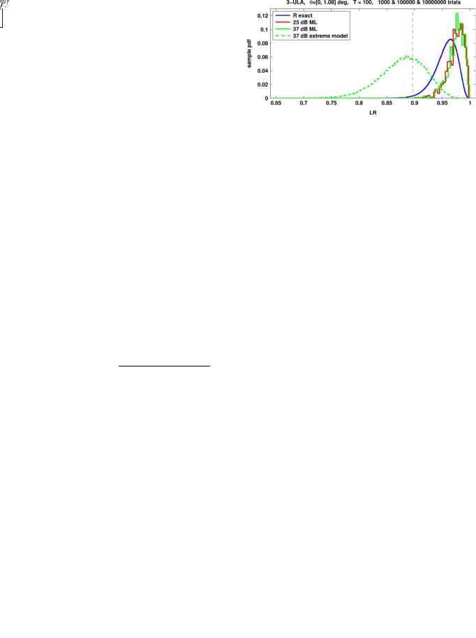
Fig. 6. Comparison of LR LR 
 and LR (R extreme model).
pdf for LR

 , and introduce some “similarity” criterion between the two pdf’s for LR

 and LR


 . Then, we can search for the extreme (in a certain sense) model that still satisfies a “similarity” criterion.
For example, the extreme model may be calculated as the two-source scenario with one source in the “center of gravity”  , while the extreme DOA for the outlier is searched for.
In result of such a development we will define an “extreme” model 
 that is statistically indistinguishable from the true covariance matrix
  (for a given
  and
and  , of course). Therefore we intend to investigate extremities of the covariance matrix model that for a limited sample support
  are statistically indistinguishable from the true covariance matrix. Indeed, if the pdfs for LR

 and LR


 overlap significantly, it means that in any specific trial, the “extreme” model
 may be found more “likely” than the true covariance matrix LR


 LR
LR

 and therefore will be selected by the MLE algorithm. We have observed this behavior in many of our MLE simulation trials. To illustrate this behavior, we collected the likelihood ratio values for the true
  and ML covariance matrix model
 in every trial and overplot these LR sample pdfs over the “theoretical” pdf for LR(R) (calculated over

 trials for


 ) in Fig. 6. As one would expect, our sample pdf’s for LR


 are right shifted with respect to the pdf for LR

 , which is the reflection of the ML property LR


 LR
LR

 . Interestingly enough, the pdfs for LR


 at SNR
  25 dB and 37 dB are practically indistinguishable, and the same behavior is observed for all analyzed scenarios. The latter observation means that not only does the pdf for LR

 not depend on
  , but it appears that the pdf of LR


 also does not depend on scenario
  , and is fully specified by
  and
and  . Accurate analytical proof of this conjecture runs beyond the scope of this paper, and we relegate it to a side observation.
In the same figure we introduce the sample pdf for LR


 calculated for the “extreme” scenario, illustrated by the right sub figure in Fig. 2. As one would expect, this pdf is left shifted with respect to LR

 . Yet, the overlap of the two pdf’s is significant enough for the event LR


 LR
LR

 to take place. Therefore, algorithmically at least, we can search for an alternative model


 or
or 


 , which for the given model


 and sample support
  , provides a required probability (


 , say) of the event LR


 LR
LR


 that may be expected to occur at least once over 1000 Monte Carlo trials. In fact, simulations in Fig. 6 specifically illustrate this
3654 |
IEEE TRANSACTIONS ON SIGNAL PROCESSING, VOL. 58, NO. 7, JULY 2010 |
methodology. Obviously, while feasible, this “algorithmic” approach is too computationally demanding, almost as demanding as the direct exhaustive search for the MLE estimate, in this case.
Alternatively, one may also consider to involve the non-asymptotic (accurate) pdfs for LR

 and LR

 . Unfortunately, even for the LR

 (7), the pdf involves Meijer’s G-functions [39], while the exact pdf for the non-null hypothesis

 is practically unmanageable since it is given in [31] as a poorly convergent series of Meijer’s G-func- tions.
For this reason, we implement our search for the extreme scenario 


 or
or 


 that is “statistically indistinguishable” from the true scenario


 , using a more computationally manageable metric of the random matrices
  and
and  “similarity,” where
(21)
This metric is provided by random matrix theory (RMT), also known as general statistical analysis (GSA, G-analysis).
B. RMT “Single Cluster” Similarity Testing Criterion
The RMT/GSA approach is to analyze asymptotic behavior of the random sample matrix eigendecomposition under the Kolmogorov asymptotic assumption 


 . RMT has established [27], [28] that the sample distribution of the covariance matrix
  eigenvalues tends almost surely to a specific pdf


 G-asymptotically. (For finite
  , this distribution


 is an approximation of the actual eigenvalue distribution). Note that
  may be equivalently introduced as
|
|
|
|
|
where |
|
(22) |
||||
Let |
. Then, the asymptotic |
||||
density of |
distinct eigenvalues in has a very special be- |
||||
havior. Specifically, as the number of training samples per an-
tenna element increases |
tends |
|
to concentrate around true eigenvalues. This is reasonable, |
||
since as |
for a fixed , the entries of |
in (22) con- |
verge to |
entries almost surely. Conversely, when the an- |
|
tenna dimension |
is high compared to a decreasing number |
of training samples |
broadens, eventually coalescing |
to only one cluster (i.e., is an uni-modal distribution).
As shown in [27], [28], if some sample eigenvalues fall in one cluster (mode) of the asymptotic density 


 , these eigenvalues are not separable, i.e., their estimates do not statistically differ. If, indeed, all sample eigenvalues fall into a single cluster of asymptotic distribution


 , then all of them are inseparable.
A key RMT result is that for the true covariance matrix 

, when |
, the empirical (sample) distribution of the |
matrix for |
converges almost surely to the nonrandom |
limiting distribution 


 specified by Marcˆenko–Pastur law [40]
(23)
where 


 and
and 

 are the extreme eigenvalues of the matrix
 .
.
Obviously, the Marcˆenko–Pastur law (23) describes a single cluster that contains all sample eigenvalues of  . Of course, for a finite
  and
and  , (23) is only an approximation, but in numerous studies (see, e.g., [41]) it was demonstrated that this convergence


 is surprisingly fast, allowing the use of the deterministic pdfs


 instead of empirical ones.
Therefore, we may consider the two random matrices  and
and 


 statistically indistinguishable if the asymptotic (deterministic) density


 for
for  is such that:
1)


 presents only a single cluster as in (23);
2)this cluster is bounded by 


 and
and 

 as in (23). If these bounds do not hold for

 , the ratio
(24)
must at least be minimal. The formulated conditions have a straightforward meaning: in order for the likelihood ratio
LR |
to be sufficiently close to the LR , the span of the |
|
eigenvalues in |
should be minimal, with the eigenvalues |
|
evenly distributed over this span. RMT is expected to provide a connection between the sample volume per antenna element ratio 


 , and the actual eigenvalues in
  , for the sample eigenvalues to stay in a single cluster.
In [27] and [28], it was demonstrated that the cluster of the specific  th eigenvalue


 is separated from the clusters associated with the adjacent eigenvalues, if and only if a so-called “eigenvalue splitting condition” is met
where |
|
|
(25) |
|
|||
is as shown in Appendix A in (A.10). |
|||
In our case, statistical nonidentifiability (ambiguity) condition a) above, requires the contrary condition, since in order for  to have all sample eigenvalues in a single cluster, none of the eigenvalues of
  can meet this “eigenvalue splitting condition.”
The following theorem presents the “inverted splitting condition” to suit our application. In sequel, we call this the “single-
cluster condition”: |
|
||||||
Theorem: Let the distinct eigenvalues of the matrix |
be |
||||||
|
|
|
|
|
|
with multiplicity |
, |
and consider |
|
||||||
|
|
|
|
|
|
|
(26) |
|
|
|
|
|
|
|
|
|
|
|
|
|
|
|
|
ABRAMOVICH AND JOHNSON: DETECTION–ESTIMATION OF VERY CLOSE EMITTERS |
3655 |
then as 


 all sample eigenvalues
 of
of  belong to a single cluster if and only if
|
|
|
|
|
(27) |
|
with |
given in Appendix A in (A.10). |
|||||
|
||||||
This |
condition |
checks whether a |
particular |
scenario |
||
|
is |
ambiguous (unresolvable) with |
respect |
|||
to the given scenario, say |
, and therefore may |
|||||
be obtained as a solution by the MLE algorithm. |
|
|||||
C. “Single Cluster”-Based Search for MLE Ambiguity Region
This condition also allows a search for an extreme scenario with parameters 


 or
or 


 where the inequality in (27) turns into equality, bounding the “MLE ambiguity region.” Between these bounds, we may consider the
two-source model with DOAs |
or |
with the power |
attributed to the source at midpoint |
and the remaining |
|
(small) power  to the second source. For any running
 or
or 
 , the power of the second source
  may be searched in the vicinity of the second large eigenvalue in
  to maximize the ratio
(28)
in the “whitened” matrix 


 . This reflects uniformity of eigenvalues in
  , as required by (24). The upper and the lower bounds for the “MLE ambiguity region”


 and
and 


 are found as the extreme DOAs


 that still meet the “single cluster” condition
(29)
Note that all calculations involve 1-D search (over  ) for each
 or
or 
 , which is relatively simple. Of course, for a more complicated scenario with

 , a search for an alternative extreme scenario my be more complicated, but if some of the

 sources are congregated in a number of clusters with poorly separated sources within, a similar approach may be applied for each of those clusters.
In some cases, illustrated below, this analysis can be completed analytically, without resorting to calculations.
Case 1—Lower Bound for the “GLRT-Based SNR Threshold Range”: Recall that the lower bound for the GLRT-based de- tection-estimation “SNR threshold range” was specified above as the SNR where the covariance matrix model built with a single source “best” DOA estimate in vicinity of the midpoint


 exceeds the LR threshold
 in (8), which means that the GLRT-based detection-estimation technique (8) treats this model as sufficiently “likely.”
Let us investigate here this SNR threshold, which means that for the given true covariance matrix 
(30)
we have to find out when the single-source model
(31)
with appropriately chosen power  , satisfies our “single cluster” criterion.
Luckily, for the two-source scenario, the exact analytical expressions for eigenvalues and eigenvectors of an  -variate covariance matrix, have been derived in [42, Ch. 5]. It appears that for two uncorrelated sources in white noise, the three different eigenvalues in
  are equal to
(32)
where the noise eigenvalue 
 has multiplicity


 , and
, and
(33)
Moreover, the eigenvector 
 that corresponds to the largest eigenvalue
 in
in  , for
, for 


 (as per our scenario), tends to
(34)
These analytical expressions reflect the anticipated fact that our scenario with the two closely located sources is practically equivalent to a scenario with one strong plane-wave source with most of the total power 


 impinging at the midpoint direction
  , and a weak source with the “wrinkled” wavefront described by the eigenvector
 of the covariance matrix
  [43]. This observation backs our assertion regarding


 in (13) being properly described by the CRB for a single source with the DOA
  and power


 . For our current study, it obviously means that the alternative single-source model is
(35)
which has the same eigenvectors as the original matrix  . The latter allows to directly calculate only two different eigenvalues of the “whitened” matrix


 that are
(36)
Calculations introduced in Appendix B reveal that the “singlecluster” condition (27) is met, if
(37)
3656 |
IEEE TRANSACTIONS ON SIGNAL PROCESSING, VOL. 58, NO. 7, JULY 2010 |
Case 2—Lower Bound for the “ITC SNR Threshold Region”:
Of course in our simulations, we have already noted that the lower bound of the “SNR threshold range,” where the singlesource model (31) becomes sufficiently likely and exceeds the LR threshold 
 , is very close to the ITC threshold


 where an ITC criterion with high probability detects the presence of a single source, instead of the true two ones.
Now we provide the RMT support for this observation. Specifically, we specify the sample support  in an
in an  -element antenna array, such that the cluster of


 noise subspace eigenvalues


 becomes inseparable from the neighboring cluster of the smallest signal subspace eigenvalue
 .
.
For 

 sources, derivations introduced in Appendix A lead to the condition
(38)
which is very close to the single-source condition in (37), especially for 

 .
.
For an arbitrary  , when the covariance matrix
  has
has 


 different eigenvalues
(39)
where the noise eigenvalue 
 has multiplicity


 , we get
(40)
which now could be viewed as the new RMT condition for ITC failure.
IV. ACCURACY OF RMT PREDICTION FOR THE “MLE
AMBIGUITY REGION”
We consider first a scenario with the “orthogonal” outlier, where 


 . This “orthogonal” scenario can be specified for arbitrary antenna geometries and may be treated as the worst case, when a set of two completely orthogonal steering vectors is frequently found to be more “likely” than the true scenario with highly linearly dependent steering vectors. In
this case, the search for the optimum power estimate |
for the |
orthogonal source at is not required since both |
and |


 are the eigenvectors of the “extreme” covariance matrix model


(41) In principle, quite straightforward, but bulky derivations allow us to analytically calculate the eigenspectrum of the whitened covariance matrix  , that has three different eigenvalues
(42)
where the eigenvalue 
 has multiplicity


 . Direct calculations for such an orthogonal outlier in

 -el- ement ULA with


 and
and 


 shows that for
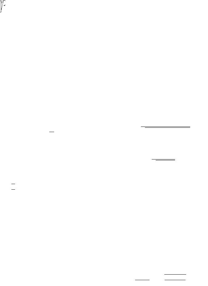
Fig. 7. General-test LR pdf for three-sensor ULA with 100 snapshots. For 37 dB, the max LR is 0.008!.
|
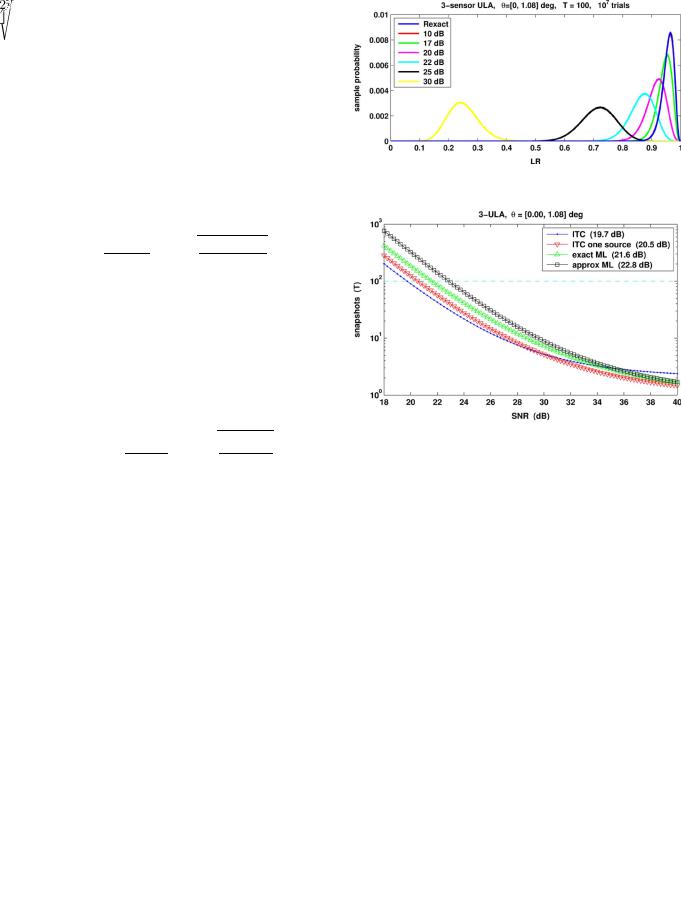
Fig. 8. ITC and GLRT breakdown for the simulated scenario. |
|
|
SNR |
dB, we get |
and |
; |
i.e., |
and |
. These eigenvalues sat- |
|
isfy the single cluster |
condition (27) and (37), namely |
||
|
|
which means that this |
sce- |
nario is within the “MLE ambiguity region.” Interestingly, the scenario with the same “orthogonal” outlier 


 but at 22-dB SNR, does not satisfy the single cluster condition since


 here, reaffirming our observation that the detection SNR threshold is around 22 dB. Further evidence of the accuracy of the single-cluster criterion is provided by analyzing sample pdfs shown in Fig. 7. Below around 10 dB, there is no practical difference between this model and the exact LR

 , whereas above 25 dB, the probability of exceeding the threshold


 rapidly vanishes. Fig. 7 shows that

 % probability lies between 20 and 22 dB. More accurate calculations are illustrated by Fig. 8, which shows that the RMT prediction for the threshold SNR is 21.6 dB (“exact ML”) for


 snapshots.
We also plot results for the single-source model (37) (GLRT one source) and the ITC threshold (40) (ITC).
The ITC threshold value of 19.7 dB agrees with the simulation results in Fig. 2, and corresponds to the point where MDL and MAP fail completely, with AIC failing in about 50% of cases. Similarly, the “GLRT single-source” SNR threshold prediction is at 20.5 dB and agrees with Fig. 5, where the LR
threshold |
is exceeded with probability of about |
for SNR |
dB. |
Therefore, the lower SNR bound within the “SNR ambiguity range” as well as the occurrence of the extreme “orthogonal”