

Holpzaphel_-_Nonlinear-Solid-Mechanics-a-Contin
.pdfAcknowledgements
When I was a postdoctoral student at Stanford University I worked with the late Juan
C. Simo, Professor of Mechanical Engineering, to whom I owe my deepest thanks. He stimulated, influenced and focused my study and writing in recent years; his friendship, versatility and dedication to scientific excellence provided a unique learning experience for me.
I am particularly indebted to Ray W. Ogden, Professor of Mathematics at the University of Glasgow, who spent a lot of time in reading the entire manuscript and rectifying certain ineptnesses. His outstanding expertise in the field made working with him an inspiring pleasure. His detailed scientific criticism and suggestions for improvements of the text were of immeasurable help.
Many others have contributed to the book. Here I mention my collaborators, whose gentle encouragement and support during the course of the preparation of the manuscript I gratefully acknowledge. In particular, the inspiring and detailed comments of
D1: Christian A.J. Schulze-Bauer, from a background in physics and medicine, were extremely helpful. He let me filter this text through his sharp mind. Also, Christian
T. Gasser, whose background is in mechanical engineering, has suggested a number of valuable improvements to the substance of the text. His profound remarks in class prevented me from getting away with anything. Also~ Elisabeth Pernkopf, a mathematician, deserves special thanks for her generous assistance. She gave much helpful advice on the preparation of this text and offered many suggestions for improving it. Special thanks are due to Michael Stadler for his productive discussions and to Mario 0. Pa/Ii for his patience in preparing the figures. I am grateful to each of these individuals without whose contributions the book would not have taken this shape.
I want to thank the Department of Civil Engineering, Graz University of Technology, for providing an environment in which this project could be completed. My gratitude goes to Gernot Beer, Professor of Civil Engineering, for his outspoken support. I also wish to acknowledge the Austrian Science Foundation, which has influenced my scientific agenda through the financial support of several grants over the past eight years.
xm

xiv |
Acknowledgements |
The enjoyment I experienced in writing this textbook would not have been the same without the moral support of numerous friends. My thanks belong to all of them who tolerated my absence when I disappeared for many evenings and weekends in order to bring the ideas of this fascinating field to you, the reader.

1 Introduction to Vectors and Tensors
The aim of this chapter is to present the fundamental rules and standard results of tensor algebra and tensor calculus permanently used in nonlinear continuum mechanics. Some readers may prefer to pass directly to Chapter 2 leaving the present part for reference as needed.
Many of the statements are given without proofs. For a more detailed exposition see the standard texts by HALMOS [1958], TRUESDELL and NOLL [1992] or the textbooks by CHADWICK [1976], GURTIN [1981a], SIMMONDS [1994], DANIELSON [1997] and OGDEN [ 1997] among many other references on vectors and tensors. To recall the
elements of linear algebra see, for example, the book by STRANG [1988a].
In this text we use lowercase Greek letters for scalars, lowercase bold-face Latin letters for vectors, uppercase bold-face Latin letters for second-order tensors, uppercase bold-face calligraphic letters for third-order tensors and uppercase blackboard
Latin letters for fourth-order tensors; for example, |
|
|
|
a, {3, (, . . . (scalars) |
a, b, c, . . . |
(vectors) |
|
|
|||
A, B, C, . . . (2nd-order tensors) |
A B, C, ... (3rd-order tensors) |
(1.1) |
|
A, Jm, C, . . . |
(4th-order tensors) . |
|
|
For equations such as |
|
|
|
u = av = {Ja = 1b |
, |
(1.2) |
|
we agree that (1.2)2 refers to u = {Ja.
Often the derivations of formulas need relations introduced previously. If this is the case we refer to these relations in a particular order, reflecting the consecutive steps necessary for deriving the formula in question.
1.1Algebra of Vectors
A physical quantity, completely described by a single real number, such as temperature, density or mass, is called a scalar designated by a, /3, ')', ... A vector designated
1

2 1 Introduction to Vectors and Tensors
by u, v, w, ... (or in other texts frequently designated by ''i',~' 1!!' ..., or fi, 'V, 'lV, ...), is a directed line element in space. It is a model for physical quantities having both direction and length, for example,force, velocity or acceleration. Two vectors that have the same direction and length are said to be equal.
The sum of vectors yields a new vector, based on the parallelogram law of addi-
tion. The following properties
u+v=v+u, |
(I .3) |
(u + v) + w = u + (v + w) , |
( 1.4) |
u+o=u, |
(1.5) |
u+ (-u) == o |
(1.6) |
hold, where o denotes the unique zero vector with unspecified direction and zero length.
Let u be a vector and a be a real number (a scalar). Then the scalar multiplication au produces a new vector with the same direction as u if a > 0 or with the opposite direction to u if n < 0.
Further properties are:
|
|
(n,B)u = o{Bu) , |
|
(1.7) |
||
|
|
(er+ f3)u = nu+ {Ju , |
|
(1.8) |
||
|
|
a(u+v)=au+o:v. |
|
( 1.9) |
||
Dot product. |
The dot (or scalar or inner) product of u and v, denoted by u · v (or |
|||||
(u, v} ), is |
|
|
|
|
|
|
|
u · v = |
lul lvlcosO(u, v) |
, |
O<O(u,v)<7r, |
|
( 1.10) |
where O(u, v) |
is the angle between two nonzero vectors u and v when their origins |
|||||
coincide. This product gives a scalar quantity with the properties |
|
|
||||
|
|
U·V |
|
V·U |
|
(I.II) |
|
|
U·O |
|
0 ' |
|
( 1.12) |
|
|
u · (nv + {3w) |
|
a(u·v)+/J(u·w) |
|
(l.13) |
U· U > 0 |
u#o |
and |
u. u = 0 |
U=O |
(l.14) |
|
The quantity lul (or !lull) is called the length (or norm or magnitude) of a vector
u, which is a non-negative real number. It is defined by the square root of u · u, i.e.
1 2 |
> o , |
') |
( 1.15) |
Iu I = (u · u) ' |
u- = u. u . |
1.1 Algebra of Vectors |
3 |
|
A vector e is called a unit vector if lel |
= 1. A nonzero vector u is said to be |
|
orthogonal (or perpendicular) to a nonzero vector v if |
|
|
with |
O(u,v) =7r/2 . |
( 1.16) |
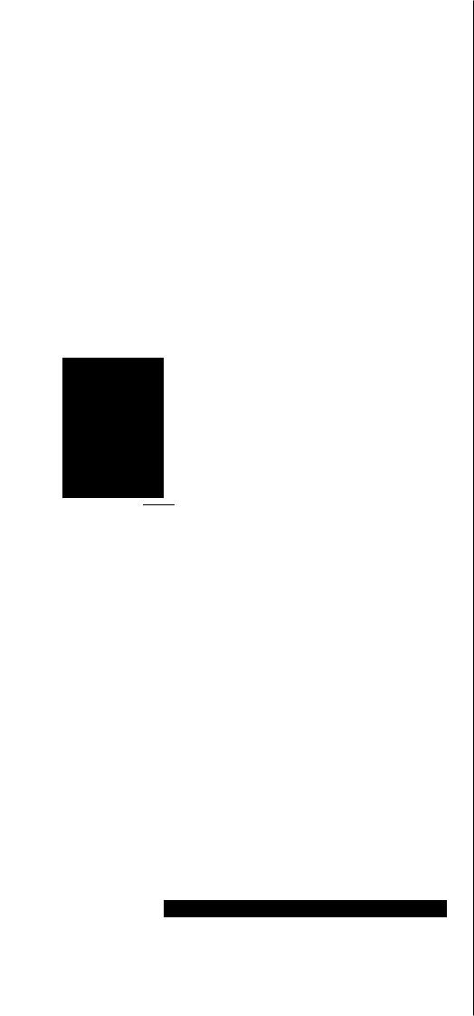
Thus, using ( l .10) we find the projection of a vector u along the direction of a
vector e with unit length, i.e. |
|
u · e == jujcosO(u, e) . |
( 1.17) |
For a geometrical interpretation of eq. ( 1. I7) see Figure I. I . |
|
u
\0 l
-~ -""------ : ~------·-
e
Figure 1.1 Projection of u along a unit vector e.
Index notation. So far algebra has been presented in symbolic (or direct or abso-
lute) notation exclusively employing bold-face letters. It represents a very convenient and concise tool to manipulate most of the relations used in continuum mechanics. It will be the preferred representation in this text. However, particularly in computational mechanics, it is essential to refer vector (and tensor) quantities to a basis. Additionally, to gain more insight in some quantities and to carry out mathematical operations among (higher-order) tensors more readily (see next section) it is often helpful to refer to components.
In order to present coordinate (or component) expressions relative to a righthanded (or dextral) and orthonormal system we introduce a fixed set of three basis vectors e1 , e2 , c:i (sometimes introduced as i,j, k), called a (Cartesian) basis, with properties
e1 |
• e., = e1 |
• e3 |
= e? · e3 |
= 0 |
' |
|
.., |
.. |
- .. |
|
These vectors of unit length which are mutually orthogonal form a so-called orthonormal system.
4 1 Introduction to Vectors and Tensors
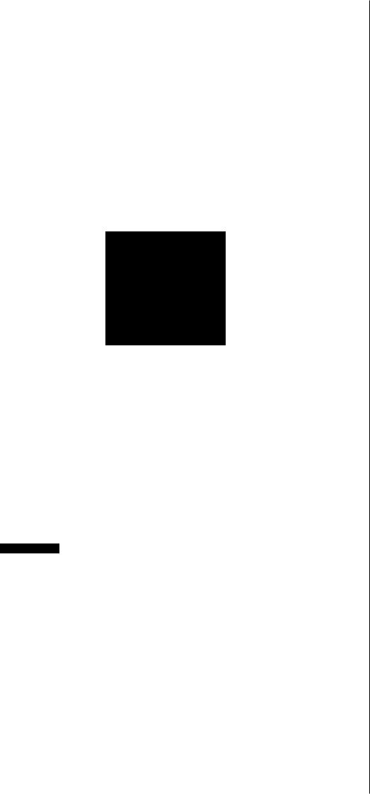
Then any vector u in the three-dimensional Euclidean space is represented uniquely by a linear combination of the basis vectors e1, e2 , e3 , i.e.
( 1.19)
where the three real numbers u1 , 'U , u3 are the uniquely determined Cartesian (or rect-
2
angular) components of vector u along the given directions e1 , e2 , e:1, respectively (see Figure 1.2). The components of e1 , e2 , e3 are (1, 0, 0), (0, 1, 0), (0, 0, 1), respectively.
u
'lL]
Figure 1.2 Vector u with its Cartesian components u 1 , u2 , u3 •
Using index (or subscript or suffix) notation, relation (l.19) can be written as u = E~=t uiei or, in an abbreviated form by leaving out the summation symbol, simply
as |
|
(sum over i = 1, 2, 3) , |
( 1.20) |
where we have adopt the summation convention, invented by Einstein. The summation convention says that whenever an index is repeated (only once) in the same term, then, a summation over the range of this index is implied unless otherwise indicated. We consider only the three-dimensional Euclidean space, which we characterize by means of Latin indices i, j, k ... running over 1, 2, 3. We denote the basis vectors by
{ ei he{ 1,2,3} collectively. Subsequently, in this text, the braces {•} will stand for a fixed set of basis vectors and the symbol • for any tensor element.
The index i that is summed over is said to be a dummy (or summation) index, since a replacement by any other symbol does not affect the value of the sum. An index that is not summed over in a given term is called a free (or live) index. Note that in the same equation an index is either dummy or free. Thus, relations ( 1.18) can be
1.1 Algebra of Vectors |
|
5 |
written in a more convenient form as |
|
|
if |
I =J |
, |
|
i # j |
( 1.2 l) |
if |
' |
|
which defines the Kronecker delta 8ii. The useful properties |
||
8ii = 3 ' |
|
(1.22) |
hold. Note that 8ii also serves as a replacement operator; for example, the index on
'Ui becomes an j when the components 'Ui are multiplied by oii·
The projection of a vector u = ·u.iei onto the basis vectors ei yields the j-th compo-
Thus, from eq. ( 1.20) and properties ( 1.13), ( 1.21) and ( l.22h we have
 ( 1.23) Taking the basis {ei} and eqs. (l.13), (l.20), (l.21) and (l.22)2, the component expres-
sion for the dot product (I. I 0) gives
u · v = u;ei ·viei = U.(Vjei ·ei = Ui'vi8ii |
= u.ivi |
= 'l1. I 'VJ + 'll2V2 + 'll:fV3 , |
( 1.24) |
which is commonly used as the definition of the dot product. Thus, we may derive the dot product of u and v without knowledge of the angle between u and v.
In an analogous manner, the component expression for the square of the length of u, i.e. ( 1.15), is
lul 2 = U· U= U;Ci • |
'lljej = U(lljc)ij = 'll(l/.; |
|
||
•) |
') |
•) |
. |
( 1.25) |
= 'llj+ ll~ |
+ 'll3 |
|||
Note that in eqs. ( 1.24) and ( 1.25) one index is repeated, indicating summation over
1, 2, 3. In symbolic notation this is indicated by one dot.
Cross product. The cross (or vector) product of u and v, denoted by u xv (in the literature also u /\ v), produces a new vector. The cross product is not commutative. It is defined as
u xv= -(v x u) |
, |
( l.26) |
|
UXV=O |
u and v are linearly dependent |
( l.27) |
|
(O'.U) X V = U X (O'.V) = ft ( U X V) , |
( 1.28) |
||
u · (v x w) = |
v · (w x u) = w ·(u x v) , |
(I .29) |
|
u x (v + w) = |
(u xv)+ (u x w) = u xv+ u x w . |
( l.30) |
|

6 1 Introduction to Vectors and Tensors
If relation (1.27) holds with u and v assumed to be nonzero vectors, we say that vector u is parallel to vector v. From eq. (1.29) we learn that
u · (u x v) = 0 . |
( l.31) |
|
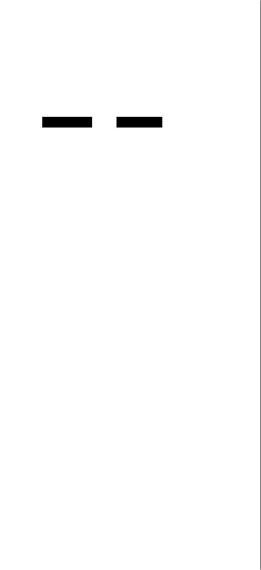
The magnitude of the cross product is defined to be |
|
|
In x vi = lnl lvlsinO(u, v) , |
0 < O(u, v) < " . |
( 1.32) |
It characterizes the area of a parallelogram spanned by the vectors u and v (see Figure 1.3). The right-handed cross product of u and v, i.e. the vector u x v, is perpendicular to the plane spanned by u and v (0 is the angle between u and v).
uxv
v
.~ Area= lox vi
I
I
I
I
I
I
: u
I
I
f
-u xv= v x u
Figure 1.3 Cross product of vectors u and v.
In order to express the cross product in terms of components we introduce the
permutation (or alternating or Levi-Civita e-) symbol C.ijk' which is defined as
C.ijk = |
|
I |
, |
for even permutations of (i, j, k) (i.e. 123, 231, 312) |
|
, |
|
|
|||||
|
- I |
' |
for odd permutations of (i, j, k) (i.e. 132, 213, 321) |
, |
( 1.33) |
|
|
|
0 |
, |
if there is a repeated index , |
|
|
with the properties Eijk = C.jki == C.kij' C.ijk = -Eiki and Eijk = -c.J'ib respectively. |
||||||
Consider the right-handed and orthonormal basis {ei}, then |
|
|
||||
|
|
|
|
e 1 x e 1 = e2 x e2 |
|
|
|
|
|
|
|
|
|
|
|
|
|
== C3 X e:1 = 0 , |
|
( 1.34) |
|
|
|
|
|
|
|
|
|
|
|
|
|
|
1.1 Algebra of Vectors |
7 |
or in a more convenient short-hand notation, with ( 1.33),
( 1.35)
With relations ( 1.2 I), ( 1.34), (1.35) it is easy to verify that EiJk may be expressed as the determinant of a matrix
( 1.36)
where we have introduced the square brackets [•] for a matrix. The product of the
permutation symbols is related to the Kronecker delta by the relation
( 1.37)
With (1.22) 1 and (l.22h we deduce from (l.37) the important relations
Eijk Eijk = 6 . ( 1.38)
EXAMPLE 1.1 Obtain the coordinate expression for the cross product w = u x v.
Solution. Taking advantage of eqs. (1.20) and ( 1.35) we find that
(l .39)
with the three components
( 1.40)
( l.41)
( 1.42)
Consequently, (u x v) · ek equals Eijk'uivi. |
• |
|
|
Now, using expressions ( 1.36), ( 1.39). , the vector product u x v relative to {ek} 1
may be written as
|
[ |
e1 |
e:! |
e:1 |
l |
|
|
|
|
|
|
||||
u xv= det |
|
|
|
= cijk 'lli'lJ.i ek |
( 1.43) |
||
|
u1 |
U2 |
'll:1 |
|
|||
|
|
'Vt |
'V2 |
'lJ3 |
|
|
|
8 1 Introduction to Vectors and Tensors
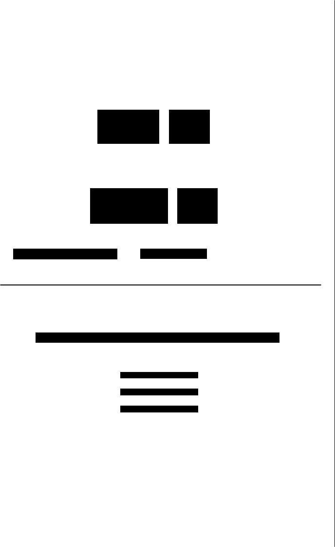
The triple scalar (or box) product (u xv)· w represents the volume F of a parallelepiped 'spanned' by u, v, w forming a right-handed triad (see Figure 1.4).
uxv
w
v
Volume= (u xv) ·w
u
Figure 1.4 Triple scalar product.
By recalling definitions ( 1.29), ( 1.10) and ( 1.32), we have
l" = (u x v) · w = (v x w) ·u = (w x u) · v |
|
= ju x vi lwlcos8 |
|
= lullvlsinO lwlcosc5 . |
( 1.44) |
~~ |
|
base area height
Using index notation, then, from eqs. ( 1.20) and (1.35) we find with ( 1.2 I) the volume
1·'"to be
l" = (u x v) · w = Eijk'lli'VfWk
= (u2'V3 - 'U;fV2}'W1 + (u3'U1 - 'UJ V:1)W2 + (u1 V2 - 'll2Vi)W:i . |
(I .45) |
Hence, the triple scalar product ( 1.45):1 can be written in the convenient determinant form
(u x v) · w = det [ :~ |
:~~ |
::~ ] |
( 1.46) |
'U3 |
'V3 |
'W3 |
|
Note that the vectors u, v, w are linearly dependent if and only if their triple scalar product vanishes (the parallelepiped has no volume).
The product u x (v x w) is called the triple vector product and may be verified with ( 1.39).i, ( 1.38)1, ( 1.22h and representations ( 1.20) and ( 1.24)4