Barro_Sala_i_Martin_2

(b)

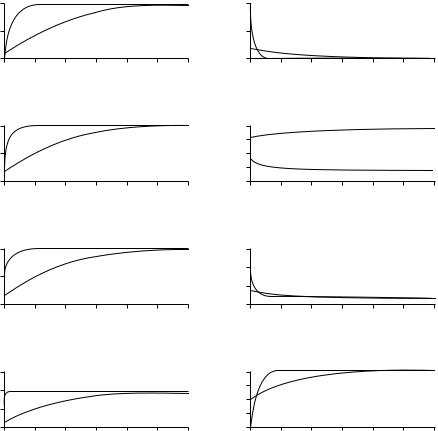
Figure 2.4

Numerical estimates of the speed of convergence in the Ramsey model. The exact speed of convergence

ˆ ˆ

(displayed on the vertical axis) is a decreasing function of the distance from the steady state, k/k (shown on the horizontal axis). The analysis assumes a Cobb–Douglas production function, with results reported for two values

of the capital share, α = 0.30 and α = 0.75. The change in the convergence speed during the transition is more

ˆ ˆ = pronounced for the smaller capital share. The value of the convergence speed, β, at the steady state (k/k 1) is

the value that we found analytically with a log-linear approximation around the steady state (equation [2.41]).

ˆ ˆ ˆ of the initial gap from k . Panel a of figure 2.5 shows how the gap between k and k is

ˆ ˆ = =

eliminated over time if the economy begins with k/k 0.1 and if α 0.3 or 0.75. As an example, if α = 0.75, it takes 38 years to close 50 percent of the gap, compared with 45 years from the linear approximation.

Panel b in figure 2.5 displays the level of consumption, expressed as cˆ/cˆ ; panel c the level of output, yˆ/yˆ ; and panel d the level of gross investment, ıˆ/ıˆ . Note that for α = 0.75, the paths of cˆ/cˆ and yˆ/yˆ are similar, because the gross saving rate and, hence, cˆ/yˆ change only by small amounts in this case (discussed later).

Panel e shows γyˆ , the growth rate of yˆ. For α = 0.3, the model has the counterfactual

about 15 percent per year, which means that γy is about 17 percent per year. This kind of result led King and Rebelo (1993) to dismiss the transitional behavior of the Ramsey model as a reasonable approximation to actual growth experiences. We see, however, that for α = 0.75, the model predicts more reasonably that γyˆ would begin at about 3.5 percent per year, so that γy would be about 5.5 percent per year.

Panel f shows the gross saving rate, s(t). We know from our previous analytical results for the Cobb–Douglas case, given the assumed values of the other parameters, that s(t)

falls monotonically when α = 0.3 and rises monotonically when α = 0.75. For α = 0.3, the

ˆ ˆ = results are counterfactual in that the model predicts a fall in s(t) from 0.28 at k/k 0.1 to

ˆ ˆ = ˆ ˆ =

0.22 at k/k 0.5 and 0.18 at k/k 1. The predicted levels of the saving rate are also unrealistically low for a broad concept of capital. In contrast, for α = 0.75, the moderate rise in the saving rate as the economy develops fits well with the data. The saving rate rises

ˆ ˆ = ˆ ˆ = ˆ ˆ =

in this case from 0.41 at k/k 0.1 to 0.44 at k/k 0.5 and 0.46 at k/k 1. The predicted level of the saving rate is also reasonable if we take a broad view of capital.

Panel g displays the behavior of the interest rate, r . Note that the steady-state interest rate is

= + = ˆ = + =

r ρ θ x 0.08, and the corresponding marginal product is f (k ) r δ 0.13. If

ˆ ˆ =

we consider the initial position k(0)/k 0.1, as in figure 2.5, the Cobb–Douglas production function implies

ˆ ˆ = ˆ ˆ α−1 = 1−α

f [k(0)]/ f (k ) [k(0)/k ] (10)

= ˆ = · ˆ =

Hence, for α 0.3, we get f [k(0)] 5 f (k ) 0.55. In other words, with a capital-

ˆ ˆ =

share coefficient of around 0.3, the initial interest rate (at k[0]/k 0.1) would take on the unrealistically high value of 60 percent. This counterfactual prediction about interest rates was another consideration that led King and Rebelo (1993) to reject the transitional dynamics of the Ramsey model. However, if we assume our preferred capital-share coefficient, α =

ˆ = · ˆ =

0.75, we get f [k(0)] 1.8 f (k ) 0.23, so that r (0) takes on the more reasonable value of 18 percent.

ˆ

The final panel in figure 2.5 shows the behavior of the capital-output ratio, (k/yˆ),

ˆ

expressed in relation to (k /yˆ ). Kaldor (1963) argued that this ratio changed relatively little during the course of economic development, and Maddison (1982, chapter 3) supported this view. These observations pertain, however, to a narrow concept of physical capital, whereas our model takes a broad perspective to include human capital. The crosscountry data show that places with higher real per capita GDP tend to have higher ratios of human capital in the form of educational attainment to physical capital (see Judson, 1998). This observation suggests that the ratio of human to physical capital would tend to rise during the transition to higher levels of real per capita GDP (see chapter 5 for a theoretical discussion of this behavior). If the ratio of physical capital to output remains relatively stable, the capital-output ratio for a broad measure of capital would increase during the transition.

a shift that departs significantly from the observed variations in k/yˆ over long periods of

= ˆ

economic development. In contrast, if α 0.75, an increase in k by a factor of 10 would

ˆ

raise k/yˆ by a factor of only 1.8. For a broad concept of capital, this behavior appears reasonable.

The main lesson from the study of the time paths in figure 2.5 is that the transitional dynamics of the Ramsey model with a conventional capital-share coefficient, α, of around 0.3 does not provide a good description of various aspects of economic development. For an economy that starts far below its steady-state position, the inaccurate predictions include an excessive speed of convergence, unrealistically high growth and interest rates, a rapidly declining gross saving rate, and large increases over time in the capital-output ratio. All of these shortcomings are eliminated if we take a broad view of capital and assume a correspondingly high capital-share coefficient, α, of around 0.75. This value of α, together with plausible values of the model’s other parameters, generate predictions that accord well with the growth experiences that we study in chapters 11 and 12.

2.6.7 Household Heterogeneity

Our analysis thus far has considered a single household as representing the entire economy. The consumption and saving decisions of the representative agent are supposed to capture the behavior of the average agent in a complex economy with many families. The important question is whether the behavior of this “representative” or “average” household is really equivalent to what we would get if we averaged the behavior of many heterogeneous families.

We can also aggregate the consumption function, equation (2.47), across households to get the economy-wide value of consumption per person:

which is the standard economy-wide condition for consumption growth. When combined with the usual analysis of competitive firms, this description of aggregate household behavior—equations (2.48) and (2.50)—delivers the standard Ramsey model. Hence, the model with the assumed forms of heterogeneity in initial assets and worker productivity has the same macroeconomic implications as the usual, representative-agent model. In other words, if the households in the economy differ in their level of wealth or productivity, and if their preferences are CIES with identical parameters and discount rates, the average consumption, assets, income, and capital for these families behave exactly as the ones of a single representative household. Hence, the representative-agent model provides the correct description of the average variables of an economy populated with the assumed forms of heterogenous agents.

Aside from supporting the use of the representative-agent framework, the extension to include heterogeneity also allows for a study of the dynamics of inequality. Equation (2.46) implies that each household chooses the same growth rate for consumption. Therefore, relative consumption, c j /c, does not vary over time.

The model does imply a dynamics for relative assets, a j /a. Equations (2.45), (2.47), (2.48), and (2.49) imply that relative assets change in accordance with

We can show that, in the steady state (where w grows at the rate x and r = ρ + θ x), the relation w = µw˜ holds. Therefore, relative asset positions stay constant in the steady state. Outside of the steady state, equation (2.51) implies that the relative asset position does not change over time for a household whose relative labor productivity, πj , is as high as its relative asset position, a j /a. For other households, the behavior depends on the sign of w − µw˜ . Imagine that w > µw˜ . Roughly speaking, this condition says that the propensity to save out of (permanent) wage income is positive. In this case, equation (2.51) implies that a j /a would rise or fall over time depending on whether relative labor productivity exceeded or fell short of the relative asset position—πj >(or <) a j /a. Thus a convergence

As has been known since Strotz (1956) and the elaborations of Pollak (1968) and Goldman (1980)—and understood much earlier by Ramsey (1928)30—nonconstancy of the rate of time preference can create a time-consistency problem. This problem arises because the relative valuation of utility flows at different dates changes as the planning date evolves. In this context, committed choices of consumption typically differ from those chosen sequentially, taking account of the way that future consumption will be determined. Therefore, the commitment technology matters for the outcomes.

Laibson (1997a, 1997b), motivated partly by introspection and partly by experimental findings, has made compelling observations about ways in which rates of time preference vary.31 He argues that individuals are highly impatient about consuming between today and tomorrow but are much more patient about choices advanced further in the future, for example, between 365 and 366 days from now. Hence, rates of time preference would be very high in the short run but much lower in the long run, as viewed from today’s perspective. Given these insights and evidence, it is important to know whether economists can continue to rely on the standard version of the neoclassical growth model—the model analyzed in this chapter—as their workhorse framework for dynamic macroeconomics.

To assess this issue, we follow the treatment in Barro (1999) and modify the utility function from equation (2.1) to

∞

U (τ ) = u[c(t)] · e−[ρ·(t−τ )+φ(t−τ )] dt (2.52)

τ

where τ now represents the current date and φ(t −τ ) is a function that brings in the aspects of time preference that cannot be described by the standard exponential factor, e−ρ·(t−τ ). For convenience, we begin with a case of zero population growth, n = 0, so that the term en·(t−τ ) does not appear in equation (2.52). We assume that the felicity function takes the usual form given in equation (2.10):

u(c) =

c(1−θ) − 1

(1 − θ)

30.In the part of his analysis that allows for time preference, Ramsey (1928, p. 439) says, “In assuming the rate of discount constant, I [mean that] the present value of an enjoyment at any future date is to be obtained by discounting it at the rate ρ. . . . This is the only assumption we can make, without contradicting our fundamental hypothesis that successive generations are activated by the same system of preferences. For, if we had a varying rate of discount—say a higher one for the first fifty years—our preference for enjoyments in 2000 A.D. over those in 2050 A.D. would be calculated at the lower rate, but that of the people alive in 2000 A.D. would be at the higher.”

31.For discussions of the experimental evidence, see Thaler (1981), Ainslie (1992), and Loewenstein and Prelec (1992).