

Barro_Sala_i_Martin_2
.pdfGrowth Models with Consumer Optimization |
105 |
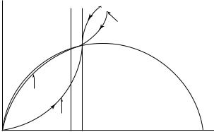
in figure 2.1. The arrows representing the dynamics of the system are also the same as before.
Since a(t) = k(t), the transversality condition from equation (2.32) can be written as
ˆ |
(2.33) |
k(T ) = 0 |
From the perspective of figure 2.1, this new transversality condition requires the initial choice of cˆ(0) to be such that the capital stock equals zero at time T . In other words, optimality now requires the economy to land on the vertical axis at exactly time T . The implication is that the stable arm is no longer the equilibrium, because it is does not lead the economy toward zero capital at time T . The same is true for any initial choice of consumption below the stable arm. The new equilibrium, therefore, features an initial value cˆ(0) that lies above the stable arm.
ˆ
It is possible that cˆ and k would both rise for awhile. In fact, if T is large, the transition path would initially be close to, but slightly above, the stable arm shown in figure 2.1.
˙ˆ = ˆ
However, the economy eventually crosses the k 0 schedule. Thereafter, cˆ and k fall, and the economy ends up with zero capital at time T . We see, therefore, that the same system of differential equations involves one equilibrium (the stable arm) or another (the path that ends up on the vertical axis at T ) depending solely on the transversality condition.
2.6.3 The Shape of the Stable Arm
ˆ 23
The stable arm shown in figure 2.1 expresses the equilibrium cˆ as a function of k. This relation is known in dynamic programming as a policy function: it relates the optimal value
ˆ
of a control variable, cˆ, to the state variable, k. This policy function is an upward-sloping curve that goes through the origin and the steady-state position. Its exact shape depends on the parameters of the model.
Consider, as an example, the effect of the parameter θ on the shape of the stable arm.
ˆ ˆ
Suppose that the economy begins with k(0) < k , so that future values of cˆ will exceed cˆ(0). High values of θ imply that households have a strong preference for smoothing consumption over time; hence, they will try hard to shift consumption from the future to
˙ˆ =
the present. Therefore, when θ is high, the stable arm will lie close to the k 0 schedule, as shown in figure 2.2. The correspondingly low rate of investment implies that the transition would take a long time.
Conversely, if θ is low, households are more willing to postpone consumption in response to high rates of return. The stable arm in this case is flat and close to the horizontal axis for
= − · ˆ
23. The corresponding relation in the Solow–Swan model, cˆ (1 s) f (k), was provided by the assumption of a constant saving rate.
106 |
Chapter 2 |
|
˙ |
˙ |
|
|
cˆt |
ˆ |
ˆ |
|
|
c 0 |
c 0 |
|
Low |
|
|
|
|
||
|
|
|
|
High |
˙ˆ k 0
 High
High
Low
ˆ* |
ˆ* |
ˆ |
k |
k |
kt |
Figure 2.2
The slope of the saddle path. When θ is low, consumers do not mind large swings in consumption over time. Hence, they choose to consume relatively little when the capital stock is low (and the interest rate is high). The investment rate is high initially in this situation, and the economy approaches its steady state rapidly. In contrast,
when θ is high, consumers are strongly motivated to smooth consumption over time. Hence, they initially devote
˙ˆ =
most of their resources to consumption (the stable arm is close to the k 0 schedule) and little to investment. In this case, the economy approaches its steady state slowly.
ˆ
low values of k (see figure 2.2). The high levels of investment imply that the transition is
ˆ ˆ
relatively quick, and as k approaches k , households increase cˆ sharply. It is clear from the diagram that linear approximations around the steady state will not capture these dynamics accurately.
We show in appendix 2C (section 2.10) for the case of a Cobb–Douglas technology,
= ˆ α ˆ ˆ ˆ
yˆ Ak , that cˆ/k is rising, constant, or falling in the transition from k(0) < k depending on whether the parameter θ is smaller than, equal to, or larger than the capital share, α. It follows that the stable arm is convex, linear, or concave depending on whether θ is smaller than, equal to, or larger than α. (We argue later that θ > α is the plausible case.) If θ = α,
ˆ
so that cˆ/k is constant during the transition, the policy function has the closed-form solution
= · ˆ + − +
cˆ (constant) k, where the constant turns out to be (δ ρ)/θ (δ n).
2.6.4 Behavior of the Saving Rate
− ˆ
The gross saving rate, s, equals 1 cˆ/f (k). The Solow–Swan model, discussed in chapter 1, assumed that s was constant at an arbitrary level. In the Ramsey model with optimizing consumers, s can follow a complicated path that includes rising and falling segments as the economy develops and approaches the steady state.
Growth Models with Consumer Optimization |
107 |
Heuristically, the behavior of the saving rate is ambiguous because it involves the offset-
ˆ ˆ ting impacts from a substitution effect and an income effect. As k rises, the decline in f (k)
lowers the rate of return, r , on saving. The reduced incentive to save—an intertemporalsubstitution effect—tends to lower the saving rate as the economy develops. Second, the
ˆ
income per effective worker in a poor economy, f (k), is far below the long-run or permanent income of this economy. Since households desire to smooth consumption, they would like to consume a lot in relation to income when they are poor; that is, the saving rate would be
ˆ ˆ
low when k is low. As k rises, the gap between current and permanent income diminishes; hence, consumption tends to fall in relation to current income, and the saving rate tends to rise. This force—an income effect—tends to raise the saving rate as the economy develops.
The transitional behavior of the saving rate depends on whether the substitution or income effect is more important. The net effect is ambiguous in general, and the path of the saving rate during the transition can be complicated. The results simplify, however, for a Cobb– Douglas production function. Appendix 2C shows for this case that, depending on parameter
ˆ
values, the saving rate falls monotonically, stays constant, or rises monotonically as k rises. We show in Appendix 2C for the Cobb–Douglas case that the steady-state saving rate,
s , is given by |
|
s = α · (x + n + δ)/(δ + ρ + θ x) |
(2.34) |
Note that the transversality condition, which led to equation (2.31), implies s < α in equation (2.34); that is, the steady-state gross saving rate is less than the gross capital share.
We can use a phase diagram to analyze the transitional behavior of the saving rate for the case of a Cobb–Douglas production function. The methodology is interesting more generally because it provides a way to study the behavior of variables of interest, such as the saving rate, that do not enter directly into the first-order conditions of the model. The method involves transformations of the variables that appear in the first-order conditions.
ˆ
The dynamic relations that we used before were written in terms of the variables cˆ and k. To study the transitional behavior of the saving rate, s = 1 − cˆ/yˆ, we want to rewrite these
ˆ
relations in terms of the variables cˆ/yˆ and k. Then we will be able to construct a phase
ˆ
diagram in terms of cˆ/yˆ and k. The stable arm of such a phase diagram will show how
cˆ/yˆ |
—and, hence, s = 1 − cˆ/yˆ |
ˆ |
—move as k increases. |
We start by noticing that the growth rate of cˆ/yˆ is given by the growth rate of cˆ minus the growth rate of yˆ. If the production function is Cobb–Douglas, the growth rate of yˆ is
|
|
|
|
|
|
|
|
|
|
ˆ |
|
|
|
|
|
|
proportional to the growth rate of k, that is, |
|
|
|
|
||||||||||||
|
1 |
|
d(cˆ/yˆ) |
|
(cˆ/cˆ) |
− |
(yˆ |
/yˆ) |
= |
(cˆ/cˆ) |
− |
α |
· |
(k˙ˆ |
/kˆ ) |
|
cˆ/yˆ · |
dt |
= |
||||||||||||||
˙ |
˙ |
|
˙ |
|
|
|
||||||||||

108 |
Chapter 2 |
We can now use the equilibrium conditions shown in equations (2.24) and (2.25) to get
1 |
· |
d(cˆ/yˆ) |
= [(1/θ) · (α Akˆ α−1 − δ − ρ − θ x)] |
|
||
|
cˆ/yˆ |
|
dt |
|
||
|
|
|
|
|
− α · [ Akˆ α−1 − (cˆ/yˆ) · Akˆ α−1 − (x + n + δ)] |
(2.35) |
where we used the equality cˆ/kˆ = (cˆ/yˆ) · Akˆ α−1. The growth rate of kˆ is |
|
|||||
k˙ˆ /kˆ |
= [ Akˆ α−1 − (cˆ/yˆ) · Akˆ α−1 − (x + n + δ)] |
(2.36) |
||||
Notice that equations (2.35) and (2.36) represent a system of differential equations in
ˆ
the variables cˆ/yˆ and k. Therefore, a conventional phase diagram can be drawn in terms of these two variables.
We start by setting equation (2.35) to zero to get the d(cˆ/yˆ) = 0 locus:
dt
cˆ/yˆ = 1 − 1 (2.37)
θα A
where ψ ≡ [(δ + ρ + θ x)/θ − α · (x + n + δ)] is a constant. This locus is upward sloping, downward sloping, or horizontal depending on whether ψ is positive, negative, or zero. The three possibilities are depicted in figure 2.3.
Independently of the value of ψ, the arrows above the d(cˆ/yˆ) = 0 locus point north, and
dt
the arrows below the schedule point south.
˙ˆ =
We can find the k 0 locus by setting equation (2.35) to zero to get
cˆ/yˆ |
= |
1 |
− |
(x + n + δ) |
· |
kˆ 1−α |
(2.38) |
|
A |
||||||||
|
|
|
|
which is unambiguously downward sloping.24 Arrows point west above the schedule and east below the schedule.
The three panels of figure 2.3 show that the steady state is saddle-path stable regardless of the value of ψ. The stable arm, however, is upward-sloping when ψ > 0, downward-sloping when ψ < 0, and horizontal when ψ = 0. Following the reasoning of previous sections, we know that an infinite-horizon economy always finds itself on the stable arm. Thus, depending on parameter values, the consumption ratio falls monotonically, stays constant,
ˆ
or rises monotonically as k rises. The saving rate, therefore, behaves exactly the opposite. A high value of θ—which corresponds to a low willingness to substitute consumption intertemporally—makes it more likely that ψ < 0 will hold, in which case the saving rate
|
ˆ |
|
d(cˆ/yˆ) |
|
|
24. When ψ < 0, the |
dk |
= 0 locus is also steeper than the |
= 0 schedule. |
||
dt |
dt |
|
|||

Growth Models with Consumer Optimization |
109 |
s |
|
|
|
|
s |
|
|
|
|
s |
|
|
|
|
|
|
|
|
|
|
|
|
|
||||||
s* |
|
|
|
|
|
|
|
|
|
|
|
|
|
|
|
|
|
|
|
|
|
|
|
|
1 |
|
|
|
|
1 |
|
|
|
|
s* 1 |
|
|
|
|
|
|
|
|
|
|
|
|
|
|
|
|
|
|
|
|
|
|
||
|
|
|
|
|
|
|
|
|
|
|
|
|
|
|
|
|
|
|
|
|
|
|
|
|
s* |
|
|
|
|
|
|
|
|
|
|
|
|
|
|
|
|
|
|
|
|
|
1 s |
* |
ˆ |
|
|
1 s |
* |
ˆ |
|
|
1 s |
* |
ˆ |
|
|
|
k |
|
|
|
k |
|
|
|
k |
|||
|
|
(a) |
|
|
|
|
(b) |
|
|
|
|
(c) |
|
|
Figure 2.3
Phase diagram for the behavior of the saving rate (in the Cobb–Douglas case). In the Cobb–Douglas case, the
ˆ
savings rate behaves monotonically. Panel a shows the phase diagram for cˆ/yˆ and k when the parameters are such that (δ + ρ + θ x)/θ > α · (x + n + δ). Since the stable arm is upward sloping, the consumption ratio increases as the economy grows toward the steady state. Hence, in this case, the saving rate (one minus the consumption rate) declines monotonically during the transition. Panel b considers the case in which (δ + ρ + θ x)/θ < α ·(x +n +δ). The stable arm is now downward sloping and, therefore, the saving rate increases monotonically during the transition. Panel c considers the case (δ + ρ + θ x)/θ + α · (x + n + δ). The stable arm is now horizonal, which means that the saving rate is constant during the transition.
is more likely to rise during the transition. This result follows because a higher θ weakens the substitution effect from the interest rate.
In the particular case where ψ = 0, the saving rate is constant at its steady-state value, s = 1/θ, during the transition. For this combination of parameters, it turns out that the wealth and substitution effects cancel out, so that the saving rate remains constant as the capital stock grows toward its steady state. Thus, the constant saving rate in the Solow– Swan model is a special case of the Ramsey model. However, even in this case, there is an important difference from the Solow–Swan model. The level of s in the Ramsey model is dictated by the underlying parameters and cannot be chosen arbitrarily. In particular, an arbitrary choice of s in the Solow–Swan model may generate results that are dynamically inefficient if s leads the economy to a steady-state capital stock that is larger than the golden rule. This outcome is impossible in the Ramsey model.
In a later discussion, we use the baseline values ρ = 0.02 per year, δ = 0.05 per year, n = 0.01 per year, and x = 0.02 per year. If we also assume a conventional capital share of α = 0.3, the value of θ that generates a constant saving rate is 17; that is, s < 1/θ applies and the saving rate falls—counterfactually—as the economy develops unless θ exceeds this high value.
110 |
Chapter 2 |
We noted for the Solow–Swan model that the theory cannot fit the evidence about speeds of convergence unless the capital-share coefficient, α, is much larger than 0.3. Values in the neighborhood of 0.75 accord better with the empirical evidence, and these high values of α are reasonable if we take a broad view of capital to include the human components. We show in the following section that the findings about α still apply in the Ramsey growth model, which allows the saving rate to vary over time. If we assume α = 0.75, along with the benchmark values of the other parameters, the value of θ that generates a constant saving rate is 1.75. That is, the gross saving rate rises (or falls) as the economy develops if θ is greater (or less) than 1.75. If θ = 1.75, the gross saving rate is constant at the value 0.57. We have to interpret this high value for the gross saving rate by including in gross saving the various expenditures that expand or maintain human capital; aside from expenses for education and training, this gross saving would include portions of the outlays for food, health, and so on.
Our reading of empirical evidence across countries is that the saving rate tends to rise to a moderate extent with per capita income during the transition. The Ramsey model can fit this pattern, as well as the observed speeds of convergence, if we combine the benchmark parameters with a value of α of around 0.75 and a value of θ somewhat above 2. The value of θ cannot be too much above 2 because then the steady-state saving rate, s , shown in equation (2.34), becomes too low. For example, the value θ = 10 implies s = 0.22, which is too low for a broad concept that includes gross saving in the form of human capital.
2.6.5 The Paths of the Capital Stock and Output
ˆ ˆ ˆ
The stable arm shown in figure 2.1 shows that, if k(0) < k , k and cˆ rise monotonically as
ˆ
they approach their steady-state values. The rising path of k implies that the rate of return,
ˆ −
r , declines monotonically from its initial position, f [k(0)] δ, to its steady-state value, ρ + θ x. Equation (2.25) and the path of decreasing r imply that the growth rate of per capita
˙ ˆ
consumption, c/c, falls monotonically. That is, the lower k(0) and, hence, yˆ(0), the higher the initial value of c˙/c.
We would also like to relate the initial per capita growth rates of capital and output, γk
ˆ
and γy , to the starting ratio, k(0). In chapter 1 we referred to the negative relations between
˙ ˆ ˙
k/k and k(0) and between y/y and yˆ(0) as convergence effects. We show in appendix 2D (section 2.11), using the consumption function from equations (2.15) and (2.16), that k˙/k declines monotonically as the economy develops and approaches the steady state. In other words, although the saving rate may rise during the transition, it cannot rise enough to
˙ ˆ
eliminate the inverse relation between k/k and k. Thus, the endogenous determination of
ˆ
the saving rate does not eliminate the convergence property for k.
Growth Models with Consumer Optimization |
111 |
We can take logs and derivatives of the production function in equation (2.18) to derive the growth rate of output per effective worker:
yˆ |
/yˆ |
= |
kˆ · f (kˆ ) |
|
· |
(kˆ |
/kˆ ) |
(2.39) |
|
f (kˆ ) |
|||||||||
˙ |
|
˙ |
|
|
|||||
ˆ
that is, the growth rate of k is multiplied by the share of gross capital income in gross product. For a Cobb–Douglas production function, the share of capital income equals the constant α. Therefore, the properties of k˙/k carry over immediately to those of y˙/y. This result applies more generally than in the Cobb–Douglas case unless the share of capital income rises fast enough as an economy develops to more than offset the fall in k˙/k.
2.6.6 Speeds of Convergence
Log-Linear Approximations Around the Steady State We want now to provide a quantitative assessment of the speed of convergence in the Ramsey model. We begin with a
ˆ
log-linearized version of the dynamic system for k and cˆ, equations (2.24) and (2.25). This approach is an extension of the method that we used in chapter 1 for the Solow–Swan model; the only difference here is that we have to deal with a two-variable system instead of a one-variable system. The advantage of the log-linearization method is that it provides a closed-form solution for the convergence coefficient. The disadvantage is that it applies only as an approximation in the neighborhood of the steady state.
Appendix 2A examines a log-linearized version of equations (2.24) and (2.25) when
expanded around the steady-state position. The results can be written as |
|
log[yˆ(t)] = e−βt · log[yˆ(0)] + (1 − e−βt ) · log(yˆ ) |
(2.40) |
where β > 0. Thus, for any t ≥ 0, log[yˆ(t)] is a weighted average of the initial and steadystate values, log[yˆ(0)] and log(yˆ ), with the weight on the initial value declining exponentially at the rate β. The speed of convergence, β, depends on the parameters of technology and preferences. For the case of a Cobb–Douglas technology, the formula for the convergence coefficient (which comes from the log-linearization around the steady-state position) is
|
= |
|
+ |
|
· |
θ |
· |
|
+ |
|
+ |
|
· |
|
|
+ α+ |
θ x |
− |
|
+ |
|
+ |
|
1/2 |
|
|
|
|
|
|
|
|
|
|
− |
|
|
||||||||||||||||
2β |
|
ζ 2 |
|
4 |
|
1 − α |
|
(ρ |
|
δ |
|
θ x) |
|
ρ |
δ |
|
(n |
|
x |
|
δ) |
|
ζ |
(2.41) |
||
|
|
|
|
|
|
|
|
|
|
|
|
|
|
|
|
|||||||||||
where ζ = ρ − n − (1 − θ) · x > 0. We discuss below the way that the various parameters enter into this formula.
112 |
Chapter 2 |
Equation (2.40) implies that the average growth rate of per capita output, y, over an interval from an initial time 0 to any future time T ≥ 0 is given by
(1/T ) |
· |
log[y(T )/y(0)] |
= |
x |
+ |
|
(1 − e−βT ) |
· |
log[yˆ |
/yˆ |
(0)] |
(2.42) |
|
T |
|||||||||||||
|
|
|
|
|
|
|
|
Hold fixed, for the moment, the steady-state growth rate x, the convergence speed β, and the averaging interval T . Then equation (2.42) says that the average per capita growth rate of output depends negatively on the ratio of yˆ(0) to yˆ . Thus, as in the Solow–Swan model, the effect of the initial position, yˆ(0), is conditioned on the steady-state position, yˆ . In other words, the Ramsey model also predicts conditional, rather than absolute, convergence.
The coefficient that relates the growth rate of y to log[yˆ /yˆ(0)] in equation (2.42), (1 − e−βT )/T , declines with T for given β. If yˆ(0) < yˆ , so that growth rates decline over time, an increase in T means that more of the lower future growth rates are averaged with the higher near-term growth rates. Therefore, the average growth rate, which enters into equation (2.42), falls as T rises. As T → ∞, the steady-state growth rate, x, dominates the average; hence, the coefficient (1 − e−βT )/T approaches 0, and the average growth rate of y in equation (2.42) tends to x.
For a given T , a higher β implies a higher coefficient (1 − e−βT )/T . (As T → 0, the coefficient approaches β.) Equation (2.41) expresses the dependence of β on the underlying parameters. Consider first the case of the Solow–Swan model in which the saving rate is constant. As noted before, this situation applies if the steady-state saving rate, s , shown in equation (2.34) equals 1/θ or, equivalently, if the combination of parameters α · (δ + n) − (δ + ρ)/θ − x · (1 − α) equals 0.
Suppose that the parameters take on the baseline values that we used in chapter 1: δ = 0.05 per year, n = 0.01 per year, and x = 0.02 per year. We also assume ρ = 0.02 per year to get a reasonable value for the steady-state interest rate, ρ + θ x. As mentioned in a previous section, for these benchmark parameter values, the saving rate is constant if α = 0.3 when θ = 17 and if α = 0.75 when θ = 1.75.
With a constant saving rate, the formula for the convergence speed, β, simplifies from equation (2.41) to the result that applied in equation (1.45) for the Solow–Swan model:
β = (1 − α) · (x + n + δ)
We noted in chapter 1 that a match with the empirical estimate for β of roughly 0.02 per year requires a value for α around 0.75, that is, in the range in which the broad nature of capital implies that diminishing returns to capital set in slowly. Lower values of x + n + δ reduce the required value of α, but plausible values leave α well above the value of around 0.3, which would apply to a narrow concept of physical capital.
Growth Models with Consumer Optimization |
113 |
In the case of a variable saving rate, equation (2.41) determines the full effects of the various parameters on the convergence speed. The new element concerns the tilt of the
ˆ
time path of the saving rate during the transition. If the saving rate falls with k, the convergence speed would be higher than otherwise, and vice versa. For example, we found before that a higher value of the intertemporal-substitution parameter, θ, makes it more likely that
ˆ
the saving rate would rise with k. Through this mechanism, a higher θ reduces the speed of convergence, β, in equation (2.41).
If the rate of time preference, ρ, increases, the level of the saving rate tends to fall (see equation [2.34]). The effect on the convergence speed depends, however, not on the level of the saving rate but on the tendency for the saving rate to rise or fall as the economy develops. A higher ρ tends to tilt downward the path of the saving rate. The effective time-preference
+ · ˙ ˙ ˆ
rate is ρ θ c/c. Because c/c is inversely related to k, the impact of ρ on the effective
ˆ
time-preference rate is proportionately less the lower is k. Therefore, the saving rate tends
ˆ
to decrease less the lower k, and, hence, the time path of the saving rate tilts downward. A higher ρ tends accordingly to raise the magnitude of β in equation (2.41).
It turns out with a variable saving rate that the parameters δ and x tend to raise β, just as they did in the Solow–Swan model. The overall effect from the parameter n becomes ambiguous but tends to be small in the relevant range.25
The basic result, which holds with a variable or constant saving rate, is that, for plausible values of the other parameters, the model requires a high value of α—in the neighborhood of 0.75—to match empirical estimates of the speed of convergence, β. We can reduce the required value of α to 0.5–0.6 if we assume very high values of θ (in excess of 10) along with a value of δ close to 0. We argued before, however, that very high values of θ make the steady-state saving rate too low, and values of δ near 0 are unrealistic. In addition, as we show later, values of α that are much below 0.75 generate counterfactual predictions about the transitional behavior of the interest rate and the capital-output ratio. We discuss in chapter 3 how adjustment costs for investment can slow down the rate of convergence, but this extension does not change the main conclusions.
Numerical Solutions of the Nonlinear System We now assess the convergence properties of the model with a second approach, which uses numerical methods to solve the nonlinear system of differential equations. This approach avoids the approximation errors inherent in linearization of the model and provides accurate results for a given specification of the underlying parameters. The disadvantage is the absence of a closed-form solution. We have to generate a new set of answers for each specification of parameter values.
25. Equation (2.41) implies that the effects on β are unambiguously negative for α and positive for δ. Our numerical computations indicate that the effects of the other parameters are in the directions that we mentioned as long as the other parameters are restricted to a reasonable range.
114 |
Chapter 2 |
We can use numerical methods to obtain a global solution for the nonlinear system of differential equations. In the case of a Cobb–Douglas production function, the growth rates
ˆ
of k and cˆ are given from equations (2.24) and (2.25) as
γkˆ |
≡ k˙ˆ /kˆ |
= A · (kˆ )α−1 − (cˆ/kˆ ) − (x + n + δ) |
(2.43) |
||||||||||||
γ |
cˆ |
cˆ/cˆ |
= |
(1/θ) |
· |
[α A |
· |
(kˆ )α−1 |
− |
(δ |
+ |
ρ |
+ |
θ x)] |
(2.44) |
|
≡ ˙ |
|
|
|
|
|
|
|
|||||||
If we specified the values of the parameters ( A, α, x, n, δ, ρ, θ) and knew the relation between
ˆ ˆ
cˆ and k along the path—that is, if we knew the policy function cˆ(k)—then standard numerical methods for solving differential equations would allow us to solve out for the entire time
ˆ
paths of k and cˆ. The appendix on mathematics shows how to use a procedure called the time-elimination method to derive the policy function numerically. (See also Mulligan and Sala-i-Martin, 1991). We assume now that we have already solved this part of the problem.
Once we know the policy function, we can determine the paths of all the variables that
= − ˆ we care about, including the convergence coefficient, defined by β d(γkˆ )/d[log(k)].
ˆ
(In the Cobb–Douglas case, the convergence coefficient for yˆ is still the same as that for k.)
ˆ ˆ
Figure 2.4 shows the relation between β and k/k when we use our benchmark parameter values (δ = 0.05, x = 0.02, n = 0.01, ρ = 0.02), θ = 3, and α = 0.3 or 0.75.26 For either
ˆ ˆ
setting of α, β is a decreasing function of k/k ; that is, the speed of convergence slows
27 ˆ ˆ =
down as the economy approaches the steady state. At the steady state, where k/k 1, the values of β—0.082 if α = 0.3 and 0.015 if α = 0.75—are those implied by equation (2.41) for the log-linearization around the steady state.
ˆ /ˆ < 1, figure 2.4 indicates that β exceeds the values implied by equation (2.41). If k k
ˆ ˆ = = = = ˆ ˆ =
For example, if k/k 0.5, β 0.141 if α 0.3 and 0.018 if α 0.75. If k/k 0.1, β = 0.474 if α = 0.3 and 0.026 if α = 0.75. Thus, if we use our preferred high value for the capital-share coefficient, α = 0.75, the convergence coefficient, β, remains between
ˆˆ
1.5percent and 3 percent for a broad range of k/k . This behavior accords with the empirical evidence discussed in chapters 11 and 12; we find there that convergence coefficients do not seem to exceed this range even for economies that are very far from their steady states.
In contrast, if we assume α = 0.3, the model incorrectly predicts extremely high rates of
ˆ ˆ convergence when k is far below k .
Since the convergence speeds rise with the distance from the steady state, the durations of the transition are shorter than those implied by the linearized model. We can use the results
ˆ
on the time path of k to compute the exact time that it takes to close a specified percentage
ˆˆ
26.For a given value of k/k , the parameter A does not affect β in the Cobb–Douglas case.
ˆ ˆ
27. This relation does not hold in general. In particular, β can rise with k/k if θ is very small and α is very large, for example, if θ = 0.5 and α = 0.95.