Note that the data includes four different columns that are based on a single date column: WageType, DayOfWeek, Shift, and DateKey. Ordinarily in data mining it is not a good idea to use multiple columns that are derived from the same data, as the values correlate with each other too strongly and can obscure other patterns.

However, we will not use DateKey in the model because it contains too many unique values. There is no direct relationship between Shift and DayOfWeek, and WageType and DayOfWeek are only partly related. If you were worried about collinearity, you could create the structure using all of the available columns, and then ignore different columns in each model and test the effect.

Next Task in Lesson

Creating a Neural Network Structure and Model

See Also

Designing Data Source Views (Analysis Services)

Creating a Neural Network Structure and Model (Intermediate Data Mining Tutorial)

To create a data mining model, you must first use the Data Mining Wizard to create a new mining structure based on the new data source view. In this task you will use the wizard to create a mining structure, and at the same time create an associated mining model that is based on the Microsoft Neural Network algorithm.

Because neural networks are extremely flexible and can analyze many combinations of inputs and outputs, you should experiment with several ways of processing the data to get the best results. For example, you might want to customize the way that the

123

numerical target for service quality is binned, or grouped, to target specific business requirements. To do this, you will add a new column to the mining structure that groups numerical data in a different way, and then create a model that uses the new column. You will use these mining models to do some exploration.

Finally, when you have learned from the neural network model which factors have the greatest impact for your business question, you will build a separate model for prediction and scoring. You will use the Microsoft Logistic Regression algorithm, which is based on the neural networks model but is optimized for finding a solution based on specific inputs.

Steps

1.Create the basic mining structure, using defaults

2.Create a copy of the predictable column and modify it by binning the values

3.Add a new model and use the new column as the output for that model

4.Create an alias for the modified predictable attribute

5.Assign a seed so that models are processed the same way; process both models

Creating the Default Call Center Structure

To create the default neural network mining structure and model

1.In Solution Explorer in SQL Server Data Tools (SSDT), right-click Mining Structures and select New Mining Structure.

2.On the Welcome to the Data Mining Wizard page, click Next.

3.On the Select the Definition Method page, verify that From existing relational database or data warehouse is selected, and then click Next.

4.On the Create the Data Mining Structure page, verify that the option Create mining structure with a mining model is selected.

5.Click the dropdown list for the option Which data mining technique do you want to use?, then select Microsoft Neural Networks.

Because the logistic regression models are based on the neural networks, you can reuse the same structure and add a new mining model.

6.Click Next.

The Select Data Source View page appears.

7.Under Available data source views, select Call Center, and click Next.

8.On the Specify Table Types page, select the Case check box next to the FactCallCenter table. Do not select anything for DimDate. Click Next.

9.On the Specify the Training Data page, select Key next to the column

FactCallCenterID.

10.Select the Predict and Input check boxes.

11.Select the Key, Input, and Predict check boxes as shown in the following table:

124

Note that multiple predictable columns have been selected. One of the strengths of the neural network algorithm is that it can analyze all possible combinations of input and output attributes. You wouldn’t want to do this for a large data set, as it could exponentially increase processing time..

12.On the Specify Columns' Content and Data Type page, verify that the grid contains the columns, content types, and data types as shown in the following table, and then click Next.

125

13.On the Create testing set page, clear the text box for the option, Percentage of data for testing. Click Next.

14.On the Completing the Wizard page, for the Mining structure name, type Call Center.

15.For the Mining model name, type Call Center Default NN, and then click Finish.

The Allow drill through box is disabled because you cannot drill through to data with neural network models.

16.In Solution Explorer, right-click the name of the data mining structure that you just created, and select Process.

Understanding Discretization

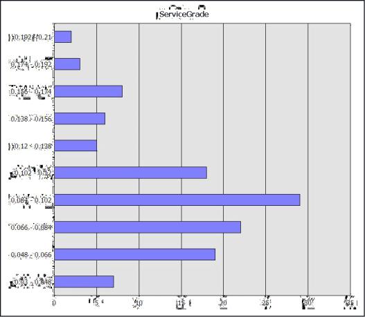
By default, when you create a neural network model that has a numeric predictable attribute, the Microsoft Neural Network algorithm treats the attribute as a continuous number. For example, the ServiceGrade attribute is a number that theoretically ranges from 0.00 (all calls are answered) to 1.00 (all callers hang up). In this data set, the values have the following distribution:

126

As a result, when you process the model the outputs might be grouped differently than you expect. For example, if you use clustering to identify the best groups of values, the algorithm divides the values in ServiceGrade into ranges such as this one: 0.0748051948 - 0.09716216215. Although this grouping is mathematically accurate, such ranges might not be as meaningful to business users. To group the numerical values differently, you can create a copy or multiple copies of the numerical data column and specify how the data mining algorithm should process the values. For example, you might specify that the algorithm divide the values into no more than five bins.

Analysis Services provides a variety of methods for binning or processing numerical data. The following table illustrates the differences between the results when the output attribute ServiceGrade has been processed three different ways:

•Treating it as a continuous number.

•Having the algorithm use clustering to identify the best arrangement of values.

•Specifying that the numbers be binned by the Equal Areas method.

127

Note

You can obtain these statistics from the marginal statistics node of the model, after all the data has been processed. For more information about the marginal statistics node, see Mining Model Content for Neural Network Models (Analysis Services - Data Mining).

In this table, the VALUE column shows you how the number for ServiceGrade has been handled. The SUPPORT column shows you how many cases had that value, or that fell in that range.

1.Use continuous numbers (default)

If you used the default method, the algorithm would compute outcomes for 120 distinct values, the mean value of which is 0.09875. You can also see the number of missing values.

2.Bin by clustering

When you let the Microsoft Clustering algorithm determine the optional grouping of values, the algorithm would group the values for ServiceGrade into five (5) ranges. The number of cases in each range is not evenly distributed, as you can see from the support column.

3.Bin by equal areas

When you choose this method, the algorithm forces the values into buckets of equal size, which in turn changes the upper and lower bounds of each range. You can

128

specify the number of buckets, but you want to avoid having two few values in any bucket.

For more information about binning options, see Discretization Methods (Data Mining).

Alternatively, rather than using the numeric values, you could add a separate derived column that classifies the service grades into predefined target ranges, such as Best (ServiceGrade <= 0.05), Acceptable (0.10 > ServiceGrade > 0.05), and Poor (ServiceGrade >= 0.10).

Creating a Copy of a Column and Changing the Discretization Method

In Analysis Services data mining, you can easily change the way that numerical data is binned within a mining structure by adding a copy of the column containing the target data and changing the discretization method.

The following procedure describes how to make a copy of the mining column that contains the target attribute, ServiceGrade. You can create multiple copies of any column in a mining structure, including the predictable attribute.

You will then customize the grouping of the numeric values in the copied column, to reduce the complexity of the groupings. For this tutorial, you will use the Equal Areas method of discretization, and specify four buckets. The groupings that result from this method are fairly close to the target values of interest to your business users.

Note

During initial exploration of data, you can also experiment with various discretization methods, or try clustering the data first.

To create a customized copy of a column in the mining structure

1.In Solution Explorer, double-click the mining structure that you just created.

2.In the Mining Structure tab, click Add a mining structure column.

3.In the Select column dialog box, select ServiceGrade from the list in Source column, then click OK.

A new column is added to the list of mining structure columns. By default, the new mining column has the same name as the existing column, with a numerical postfix: for example, ServiceGrade 1. You can change the name of this column to be more descriptive.

You will also specify the discretization method.

4.Right-click ServiceGrade 1 and select Properties.

5.In the Properties window, locate the Name property, and change the name to

Service Grade Binned .

6.A dialog box appears asking whether you want to make the same change to the name of all related mining model columns. Click No.

7.In the Properties window, locate the section Data Type and expand it if

129

necessary.

8. Change the value of the property Content from Continuous to Discretized.

The following properties are now available. Change the values of the properties as shown in the following table:

Note

The default value of

P:Microsoft.AnalysisServices.ScalarMiningStructureColumn.DiscretizationBu cketCount is actually 0, which means that the algorithm automatically determines the optimum number of buckets. Therefore, if you want to reset the value of this property to its default, type 0.

9.In Data Mining Designer, click the Mining Models tab.

Notice that when you add a copy of a mining structure column, the usage flag for the copy is automatically set to Ignore. Usually, when you add a copy of a column to a mining structure, you would not use the copy for analysis together with the original column, or the algorithm will find a strong correlation between the two columns that might obscure other relationships.

Adding a New Mining Model to the Mining Structure

Now that you have created a new grouping for the target attribute, you need to add a new mining model that uses the discretized column. When you are done, the CallCenter mining structure will have two mining models:

•The mining model, Call Center Default NN, handles the ServiceGrade values as a continuous range.

•You will create a new mining model, Call Center Binned NN, that uses as its target outcomes the values of the ServiceGrade column, distributed into four buckets of equal size.

To add a mining model based on the new discretized column

1.In Solution Explorer, right-click the mining structure that you just created, and select Open.

2.Click the Mining Models tab.

3.Click Create a related mining model.

4.In the New Mining Model dialog box, for Model name, type Call Center

130

Binned NN. In the Algorithm name dropdown list, select Microsoft Neural Network.

5.In the list of columns contained in the new mining model, locate ServiceGrade, and change the usage from Predict to Ignore.

6.Similarly, locate ServiceGrade Binned, and change the usage from Ignore to

Predict.

Ordinarily you cannot compare mining models that use different predictable attributes. However, you can create an alias for a mining model column. That is, you can rename the column, ServiceGrade Binned, within the mining model so that it has the same name as the original column. You can then directly compare these two models in an accuracy chart, even though the data is discretized differently.

To add an alias for a mining structure column in a mining model

1.In the Mining Models tab, under Structure, select ServiceGrade Binned.

Note that the Properties window displays the properties of the object, ScalarMiningStructure column.

2.Under the column for the mining model, ServiceGrade Binned NN, click the cell corresponding to the column ServiceGrade Binned.

Note that now the Properties window displays the properties for the object, MiningModelColumn.

3.Locate the Name property, and change the value to ServiceGrade.

4.Locate the Description property and type Temporary column alias. The Properties window should contain the following information:

5.Click anywhere in the Mining Model tab.

The grid is updated to show the new temporary column alias, ServiceGrade, beside the column usage. The grid containing the mining structure and two mining models should look like the following:

131

Processing the Model

Finally, to ensure that the models you have created can be easily compared, you will set the seed parameter for both the default and binned models. Setting a seed value guarantees that each model starts processing the data from the same point.

Note

If you do not specify a numeric value for the seed parameter, SQL Server Analysis Services will generate a seed based on the name of the model. Because the models always have different names, you must set a seed value to ensure that they process data in the same order.

To specify the seed and process the models

1.In the Mining Model tab, right-click the column for the model named Call Center - LR, and select Set Algorithm Parameters.

2.In the row for the HOLDOUT_SEED parameter, click the empty cell under Value, and type 1. Click OK. Repeat this step for each model associated with the

132