Advanced Time Series Predictions (Intermediate Data Mining Tutorial)

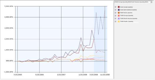
You saw from exploring the forecasting model that although sales in most of the regions follow a similar pattern, some regions and some models, such as the M200 model in the Pacific region, exhibit very different trends. This does not surprise you, as you know that differences among regions are common and can be caused by many factors, including marketing promotions, inaccurate reporting, or geopolitical events.

However, your users are asking for a model that can be applied worldwide. Therefore, to minimize the effect of individual factors on projections, you decide to build a model that is based on aggregated measures of worldwide sales. You can then use this model to make predictions for each individual region.

In this task, you will build all the data sources that you need to perform the advanced prediction tasks. You will create two data source views for use as inputs to the prediction query, and one data source view to use in building a new model.

Steps

1.Prepare the extended sales data (for prediction)

2.Prepare the aggregated data (for building the model)

3.Prepare the series data (for cross-prediction)

4.Predict using EXTEND

5.Create the cross-prediction model

6.Predict using REPLACE

7.Review the new predictions

Creating the New Extended Sales Data

To update your sales data, you will need to get the latest sales figures. Of particular interest are the data just in from the Pacific region, which launched a regional sales promotion to call attention to the new stores and raise awareness of their products.

For this scenario, we’ll assume that the data has been imported from an Excel workbook that contains just three months of new data for a couple of regions. You’ll create a table for the data using a Transact-SQL script, and then define a data source view to use for prediction.

Create the table with new sales data

1.In a Transact-SQL query window, execute the following statement to add the sales data to the AdventureWorksDW database (or any other database).

USE [database name];

GO

IF OBJECT_ID ([dbo].[NewSalesData]) IS NOT NULL

67

DROP TABLE [dbo].[NewSalesData];

GO

CREATE TABLE [dbo].[NewSalesData]( [Series] [nvarchar](255) NULL, [NewDate] [datetime] NULL, [NewQty] [float] NULL, [NewAmount] [money] NULL

) ON [PRIMARY]

GO

2. Insert the new values using the following script.

INSERT INTO [NewSalesData] (Series,NewDate,NewQty,NewAmount)

VALUES('T1000 Pacific', '7/25/08', 55, '$130,170.22'), ('T1000 Pacific', '8/25/08', 50, '$114,435.36 '), ('T1000 Pacific', '9/25/08', 50, '$117,296.24 '), ('T1000 Europe', '7/25/08', 37, '$88,210.00 '), ('T1000 Europe', '8/25/08', 41, '$97,746.00 '), ('T1000 Europe', '9/25/08', 37, '$88,210.00 '), ('T1000 North America', '7/25/08', 69, '$164,500.00 '), ('T1000 North America', '8/25/08', 66, '$157,348.00 '), ('T1000 North America', '9/25/08', 58, '$138,276.00 '), ('M200 Pacific', '7/25/08', 65, '$149,824.35'),

('M200 Pacific', '8/25/08', 54, '$124,619.46'), ('M200 Pacific', '9/25/08', 61, '$141,143.39'), ('M200 Europe', '7/25/08', 75, '$173,026.00'), ('M200 Europe', '8/25/08', 76, '$175,212.00'), ('M200 Europe', '9/25/08', 84, '$193,731.00'), ('M200 North America', '7/25/08', 94, '$216,916.00'), ('M200 North America', '8/25/08', 94, '$216,891.00'), ('M200 North America', '9/25/08', 91,'$209,943.00');

Warning

The quotation marks are used with the currency values to prevent problems with the comma separator and the currency symbol. You could also pass in the currency

68

values in this format: 130170.22

Note that the dates used in the sample database have changed for this release. If you are using an earlier edition of AdventureWorks, you might need to adjust the inserted dates accordingly.

Create a data source view using the new sales data

1.In Solution Explorer, right-click Data Source Views, and then select New Data Source View.

2.In the Data Source View wizard, make the following selections: Data Source: Adventure Works DW Multidimensional 2012

Select Tables and Views: Select the table that you just created, NewSalesData.

3.Click Finish.

4.In the Data Source View design surface, right-click NewSalesData, and then select Explore Data to verify the data.

Warning

You will use this data for prediction only, so it does not matter that the data is incomplete.

Creating the Data for the Cross-Prediction Model

The data that was used in the original forecasting model was already grouped somewhat by the view vTimeSeries, which collapsed several bike models into a smaller number of categories, and merged results from individual countries into regions. To create a model that can be used for world-wide projections, you will create some additional simple aggregations directly in the Data Source View Designer. The new data source view will contain just a sum and an average of the sales of all products for all regions.

After you have created the data source used for the model, you must create a new data source view to use for prediction. For example, if you want to predict sales for Europe using the new worldwide model, you must feed in data for the Europe region only. So you will set up a new data source view that filters the original data, and change the filter condition for each set of prediction queries.

To create the model data using a custom data source view

1.In Solution Explorer, right-click Data Source Views, and then select New Data Source View.

2.On the welcome page of the wizard, click Next.

3. On the Select Data Source page, select Adventure Works DW Multidimensional 2012 , and then click Next.

4.In the page, Select Tables and Views, do not add any tables—just click Next.

5.On the page, Completing the Wizard, type the name AllRegions, and then click

69

Finish.

6.Next, right-click the blank data source view design surface, and then select New Named Query.

7.In the Create Named Query dialog box, for Name, type AllRegions, and for

Description, type Sum and average of sales for all models and regions.

8.In the SQL text pane, type the following statement and then click OK:

SELECT ReportingDate,

SUM([Quantity]) as SumQty, AVG([Quantity]) as AvgQty, SUM([Amount]) AS SumAmt, AVG([Amount]) AS AvgAmt, 'All Regions' as [Region]

FROM dbo.vTimeSeries GROUP BY ReportingDate

9. Right-click the AllRegions table, and then select Explore Data.

To create the series data for cross-prediction

1.In Solution Explorer, right-click Data Source Views, and then select New Data Source View.

2.In the Data Source View wizard, make the following selections: Data Source: Adventure Works DW Multidimensional 2012 Select Tables and Views: Do not select any tables

Name: T1000 Pacific Region

3.Click Finish.

4.Right-click the empty design surface for T1000 Pacific Region.dsv, and then select New Named Query.

The Create Named Query dialog box appears. Retype the name, and then add the following description:

Name: T1000 Pacific Region

Description: Filter vTimeSeries by region and model

5.In the text pane, type the following query, and then click OK:

SELECT ReportingDate, ModelRegion, Quantity, Amount

FROM dbo.vTimeSeries

WHERE (ModelRegion = N'T1000 Pacific')

Note

Since you will need to create predictions for each series separately, you might want to copy the query text and save it to a text file so that you can re-use it for the other data series.

70

6.In the Data Source View design surface, right-click T1000 Pacific, and then select Explore Data to verify that the data is filtered correctly.

You will use this data as the input to the model when creating cross-prediction queries.

Next Task in Lesson

Understanding Trends in the Time Series Model (Intermediate Data Mining Tutorial)

See Also

Microsoft Time Series Algorithm (Analysis Services - Data Mining)

Microsoft Time Series Algorithm Technical Reference (Analysis Services - Data Mining) Designing Data Source Views (Analysis Services)

Time Series Predictions using Updated Data (Intermediate Data Mining Tutorial)

Creating Predictions using the Extended Sales Data

In this lesson, you will create a prediction query that adds the new sales data to the model. By extending the model with new data, you can get up-to-date predictions that include the newest data points.

Creating time series predictions that use new data is easy: you simply add the parameter EXTEND_MODEL_CASES to the PredictTimeSeries (DMX) function, specify the source of the new data, and specify how many predictions you want to get.

Warning

The parameter EXTEND_MODEL_CASES is optional; by default the model is extended any time that you create a time series prediction query by joining new data as inputs.

To build the prediction query and add new data

1.If the model is not already open, double-click the Forecasting structure, and in Data Mining Designer, click the Mining Model Prediction tab.

2.In the Mining Model pane, the model Forecasting should already be selected. If it is not selected, click Select Model, and then select the model, Forecasting.

3.In the Select Input Table(s) pane, click Select Case Table.

From the list of data source views, select NewSalesData and then click OK.

5.Right-click the surface of the design area and select Modify Connections.

6.Using the Modify Mapping dialog box, map the columns in the model to the columns in the external data as follows:

71

•Map the ReportingDate column in the mining model to the NewDate column in the input data.

•Map the Amount column in the mining model to the NewAmount column in the input data.

•Map the Quantity column in the mining model to the NewQty column in the input data.

•Map the ModelRegion column in the mining model to the Series column in the input data.

7.Now you will build the prediction query.

First, add a column to the prediction query to output the series the prediction applies to.

a.In the grid, click the first empty row, under Source, and then select Forecasting.

b.In the Field column, select Model Region and for Alias, type Model Region.

8.Next, add and edit the prediction function.

a.Click an empty row, and under Source, select Prediction Function.

b.For Field, select PredictTimeSeries.

c.For Alias, type Predicted Values.

d.Drag the field Quantity from the Mining Model pane into the

Criteria/Argument column.

e.In the Criteria/Argument column, after the field name, type the following text: 5,EXTEND_MODEL_CASES

The complete text of the Criteria/Argument text box should be as follows:

[Forecasting].[Quantity],5,EXTEND_MODEL_CASES

9.Click Results and review the results.

The predictions begin in July (the first time slice after the end of the original data) and end at November (the fifth time slice after the end of the original data).

You can see that to use this type of prediction query effectively, you need to know when the old data ends, as well as how many time slices there are in the new data.

For example, in this model, the original data series ended in June, and the data is for the months of July, August, and September.

Predictions that use EXTEND_MODEL_CASES always begin at the end of the original data series. Therefore, if you want to get only the predictions for the unknown months, you need to specify the starting point and the end point for prediction. Both values are specified as a number of time slices starting at the end of the old data.

The following procedure demonstrates how to do this.

Procedures

72

Change the start and end points of the predictions

1.In Prediction Query Builder, click Query to switch to DMX view.

2.Locate the DMX statement that contains the PredictTimeSeries function and change it as follows:

PredictTimeSeries([Forecasting 12].[Quantity],4,6,EXTEND_MODEL_CASES)

3.Click Results and review the results.

Now the predictions begin at October (the fourth time slice, counting from the end of the original data) and end at December (the sixth time slice, counting from the end of the original data).

Next Task in Lesson

Predicting using the Averaged Forecasting Model (Intermediate Data Mining Tutorial)

See Also

Microsoft Time Series Algorithm Technical Reference (Analysis Services - Data Mining) Mining Model Content for Time Series Models (Analysis Services - Data Mining)

Time Series Predictions using Replacement Data (Intermediate Data Mining Tutorial)

In this task, you will build a new model based on worldwide sales data. Then, you will create a prediction query that applies the worldwide sales model to one of the individual regions.

Building a General Model

Remember that your analysis of the results of the original mining model revealed big differences between regions and between product lines. For example, sales in North America were strong for the M200 model, while sales of the T1000 model did not do as well. However, the analysis is complicated by the fact that some series didn’t have much data, or data started at a different point in time. Some data was also missing.

73

To address some of the data quality issues, you decide to merge the data from sales around the world, and use that set of general sales trends to build a model that can be applied to predict future sales in any region.

When you create predictions, you will use the pattern that is generated by training on worldwide sales data, but you will replace the historical data points with the sales data for each individual region. That way, the shape of the trend is preserved but the predicted values are aligned with the historical sales figures for each region and model.

Performing Cross-Prediction with a Time Series Model

The process of using data from one series to predict trends in another series is called cross-prediction. You can use cross-prediction in many scenarios: for example, you might decide that television sales are a good predictor of overall economic activity, and apply a model trained on television sales to general economic data.

In SQL Server Data Mining, you perform cross-prediction by using the parameter REPLACE_MODEL_CASES within the arguments to the function, PredictTimeSeries (DMX).

In the next task, you will learn how to use REPLACE_MODEL_CASES. You will use the merged world sales data to build a model, and then create a prediction query that maps the general model to the replacement data.

It is assumed that you are familiar with how to build data mining models by now, and so the instructions for building the model has been simplified.

To build a mining structure and mining model using the aggregated data

1.In Solution Explorer, right-click Mining Structures, and then select New Mining Structure to start the Data Mining Wizard.

74

2.In the Data Mining Wizard, make the following selections:

•Algorithm: Microsoft Time Series

•Use the data source that you built earlier in this advanced lesson as the source for the model. See Advanced Time Series Prediction.

Data source view: AllRegions

•Choose the following columns for the series key and time key: Key time: ReportingDate

Key: Region

•Choose the following columns for Input and Predict: SumQty

SumAmt AvgAmt AvgQty

•For Mining structure name, type: All Regions

•For Mining model name, type: All Regions

3.Process the new structure and the new model.

To build the prediction query and map the replacement data

1.If the model is not already open, double-click the AllRegions structure, and in Data Mining Designer, click the Mining Model Prediction tab.

2.In the Mining Model pane, the model AllRegions should already be selected. If it is not selected, click Select Model, and then select the model, AllRegions.

3.In the Select Input Table(s) pane, click Select Case Table.

4.In the Select Table dialog box, change the data source to T1000 Pacific Region, and then click OK.

5.Right-click the join line between the mining model and the input data and select Modify Connections. Map the data in the data source view to the model as follows:

a.Verify that the ReportingDate column in the mining model is mapped to the ReportingDate column in the input data.

b.In the Modify Mapping dialog box, in the row for the model column AvgQty, click under Table Column and then select T1000 Pacific.Quantity. Click OK.

This step maps the column you created in the model for predicting average quantity to the actual data from the T1000 series for sales quantity.

c.Do not map the column Region in the model to any input column.

Because the model aggregated the data across all series, there is no match for the series values such as T1000 Pacific, and an error is raised when the

75

prediction query runs.

6.Now you will build the prediction query.

First, add a column to the results that outputs the AllRegions label from the model together with the predictions. This way you know that the results were based on the general model.

a.In the grid, click the first empty row, under Source, and then select AllRegions mining model.

b.For Field, select Region.

c.For Alias, type Model Used.

7.Next, add another label to the results, so that you can see which series the prediction is for.

a.Click an empty row, and under Source, select Custom Expression.

b.In the Alias column, type ModelRegion.

c.In the Criteria/Argument column, type 'T1000 Pacific'.

8.Now you will set up the cross-prediction function.

a.Click an empty row, and under Source, select Prediction Function.

b.In the Field column, select PredictTimeSeries.

c.For Alias, type Predicted Values.

d.Drag the field AvgQty from the Mining Model pane into the Criteria/Argument column by using the drag and drop operation.

e.In the Criteria/Argument column, after the field name, type the following text: ,5, REPLACE_MODEL_CASES

The complete text of the Criteria/Argument text box should be as follows:

[AllRegions].[AvgQty],5,REPLACE_MODEL_CASES

9.Click Results.

Creating the Cross-Prediction Query in DMX

You might have noticed a problem with cross-prediction: namely, that to apply the general model to a different data series, such as the T1000 product model in the North America region, you must create a different query for each series, so that you can map the each set of inputs to the model.

However, rather than building the query in the designer, you can switch to DMX view and edit the DMX statement that you created. For example, the following DMX statement represents the query that you just built:

SELECT

([All Regions].[Region]) as [Model Used], ('T-1000 Pacific') as [ModelRegion],

76

(PredictTimeSeries([All Regions].[Avg Qty],5, REPLACE_MODEL_CASES)) as [Predicted Quantity]

FROM [All Regions] PREDICTION JOIN

OPENQUERY([Adventure Works DW2003R2], 'SELECT [ReportingDate] FROM

(

SELECT ReportingDate, ModelRegion, Quantity, Amount FROM dbo.vTimeSeries

WHERE (ModelRegion = N''T1000 Pacific'')

ON

[All Regions].[Reporting Date] = t.[ReportingDate] AND

[All Regions].[Avg Qty] = t.[Quantity]

To apply this to a different model, you simply edit the query statement to replace the filter condition and to update the labels associated with each result.

For example, if you change the filter conditions and column labels by replacing 'Pacific' with 'North America', you will get predictions for the T1000 product in North America, based on the patterns in the general model.

Next Task in Lesson

Comparing Predictions for Forecasting Models (Intermediate Data Mining Tutorial)

See Also

Querying a Time Series Model (Analysis Services - Data Mining) PredictTimeSeries (DMX)

Comparing Predictions for Forecasting Models (Intermediate Data Mining Tutorial)

In the previous steps of this tutorial, you created multiple time series models:

•Predictions for each combination of region and model, based only on data for the individual model and region.

•Predictions for each region, based on updated data.

•Predictions for all models on a worldwide basis, based on aggregated data.

•Predictions for the M200 model in the North America region, based on the aggregated model.

77

To summarize the features for time series predictions, you will review the changes to see how the use of the options to extend or replace data affected forecasting results.

EXTEND_MODEL_CASES

REPLACE_MODEL_CASES

Comparing the Original Results with Results after Adding Data

Let’s look at the data for just the M200 product line in the Pacific region, to see how updating the model with new data affects the results. Remember that the original data series ended in June 2004, and we obtained new data for July, August, and September.

•The first column shows the new data that was added.

•The second column shows the forecast for July and later based on the original data series.

•The third column shows the forecast based on the extended data.

You will note that the forecasts using the extended data (shown here in bold) repeat the real data points exactly. The repetition is by design. As long as there are real data points to use, the prediction query will return the actual values, and output new prediction values only after the new actual data points have been used up.

In general, the algorithm weights the changes in the new data more strongly than data from the beginning of the model data. However, in this case, the new sales figures represent an increase of only 20-30 percent over the previous period, so there only was a slight uptick in projected sales, after which the sales projections drop again, more in line with the trend in the months before the new data.

Comparing the Original and Cross-Prediction Results

Remember that the original mining model revealed big differences between regions and between product lines. For example, sales for the M200 model were very strong, while sales for the T1000 model were fairly low across all regions. Moreover, some series didn’t have much data. Series were ragged, meaning they didn’t have the same starting point.

78

So how did the predictions change when you made your projections based on the general model, which was based on world-wide sales, rather than the original data sets? To assure yourself that you have not lost any information or skewed the predictions, you can save the results to a table, join the table of predictions to the table of historical data, and then graph the two sets of historical data and predictions.

The following diagram is based on just one product line, the M200. The graph compares the predictions from the initial mining model against the predictions using the aggregated mining model.

79