

Lectures_micro / Microeconomics_presentation_Chapter_14
.pdfthe Demand Curves of a Perfectly
Producer and a Monopolist
(a) Demand Curve of an Individual |
(b) Demand Curve of a Monopolist |
Perfectly Competitive Producer |
Price |
Price |
Market price
DM
Quantity |
Quantity |


 How a Monopolist Maximizes Profit
An increase in production by a monopolist has two opposing effects on revenue:
A quantity effect. One more unit is sold, increasing total revenue by the price at which the unit is sold.
A price effect. In order to sell the last unit, the monopolist must cut the market price on all units sold. This decreases total revenue.
The quantity effect and the price effect are illustrated by the two shaded areas in panel (a) of the following figure based on the numbers on the table accompanying it.

A and
Demand
Price, cost, marginal revenue of demand
Quantity e $500
Price e ect = -$450
 10
10
Marginal revenue = $50
–400
Total Revenue
Quantity e ect dominates |
Price e |
|
price e ect. |
||
e ect. |
||
|
||
3,000 |
|
|
1,000 |
|
Quantity of diamonds

The Monopolist’s Demand Curve and Marginal
Revenue
Due to the price effect of an increase in output, the marginal revenue curve of a firm with market power always lies below its demand curve. So a profitmaximizing monopolist chooses the output level at which marginal cost is equal to marginal revenue— not to price.
As a result, the monopolist produces less and sells its output at a higher price than a perfectly competitive industry would. It earns a profit in the short run and the long run.

The Monopolist’s Demand Curve and Marginal
Revenue
To emphasize how the quantity and price effects offset each other for a firm with market power, notice the hill-shaped total revenue curve.
This reflects the fact that at low levels of output, the quantity effect is stronger than the price effect: as the monopolist sells more, it has to lower the price on only very few units, so the price effect is small.
As output rises beyond 10 diamonds, total revenue actually falls. This reflects the fact that at high levels of output, the price effect is stronger than the quantity effect: as the monopolist sells more, it now has to lower the price on many units of output, making the price effect very large.

The Monopolist’s Profit-Maximizing Output and
Price
To maximize profit, the monopolist compares marginal cost with marginal revenue.
If marginal revenue exceeds marginal cost, De Beers increases profit by producing more; if marginal revenue is less than marginal cost, De Beers increases profit by producing less. So the monopolist maximizes its profit by using the optimal output rule:
At the monopolist’s profit-maximizing quantity of output:
MR = MC

The Monopolist’s
Output and Price
Price, cost, marginal revenue of demand
Monopolist’s optimal point
Perfectly competitive industry’s optimal point
0
of diamonds
–400


 Monopoly Versus Perfect Competition
P = MC at the perfectly competitive firm’s profitmaximizing quantity of output
P > MR = MC at the monopolist’s profit-maximizing quantity of output
Compared with a competitive industry, a monopolist does the following:
Produces a smaller quantity: QM < QC
Charges a higher price: PM > PC
Earns a profit
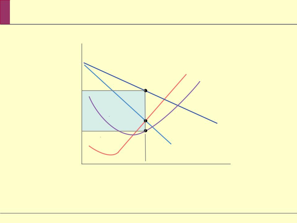

 The Monopolist’s
Price, cost, |
marginal |
revenue |
MC |
AT C |
Monopoly |
pro"t |
MR |
Quantity |
M |


 Monopoly and Public Policy
By reducing output and raising price above marginal cost, a monopolist captures some of the consumer surplus as profit and causes deadweight loss. To avoid deadweight loss, government policy attempts to prevent monopoly behavior.
When monopolies are “created” rather than natural, governments should act to prevent them from forming and break up existing ones.
The government policies used to prevent or eliminate monopolies are known as antitrust policy.