1.6. THE 2D LAPLACE EIGENVALUE PROBLEM

Добавил:

Upload Опубликованный материал нарушает ваши авторские права? Сообщите нам.

Вуз:

Санкт-Петербургский государственный электротехнический университет "ЛЭТИ"

Предмет:

[НЕСОРТИРОВАННОЕ]

Файл:

Lecture Notes on Solving Large Scale Eigenvalue Problems.pdf

Скачиваний:

Добавлен:

22.03.2016

Размер:

2.32 Mб

Скачать

☆

<<< < Предыдущая 1 2 3 45 / 635 6 7 8 9 10 11 12 13 14 15 16 17 18 19 20 21 22 23 24 25 > Следующая >>>

Figure 1.5: Triangulation of a domain Ω

T1, · · · , TN , so-called elements, such that

Ti ∩ Tj = for all i 6= j, and

Ti ∩ Tj = for all i 6= j, and

1.6Numerical methods for solving the Laplace eigenvalue problem in 2D

In this section we again consider the eigenvalue problem

(1.40)			− u(x) = λu(x),		x Ω,
with the more general boundary conditions
(1.41)			u(x) = 0,	x C1 ∂Ω,
(1.42)		∂u	(x) + α(x)u(x) = 0,		x C2 ∂Ω.

	∂n

Here, C1 and C2 are disjoint subsets of ∂Ω with C1 C2 = ∂Ω. We restrict ourselves in the following on two-dimensional domains and write (x, y) instead of (x1, x2).

In general it is not possible to solve a problem of the form (1.40)–(1.42) exactly (analytically). Therefore, one has to resort to numerical approximations. Because we cannot compute with inﬁnitely many variables we have to construct a ﬁnite-dimensional eigenvalue problem that represents the given problem as well as possible, i.e., that yields good approximations for the desired eigenvalues and eigenvectors. Since ﬁnite-dimensional eigenvalue problem only have a ﬁnite number of eigenvalues one cannot expect to get good approximations for all eigenvalues of (1.40)–(1.42).

Two methods for the discretization of eigenvalue problems of the form (1.40)–(1.42) are the Finite Di erence Method [6, 9] and the Finite Element Method (FEM) [8, 5]. We brieﬂy introduce these methods in the following subsections.

1.6.1The ﬁnite di erence method

In this section we just want to mediate some impression what the ﬁnite di erence method is about. Therefore we assume for simplicity that the domain Ω is a square with sides of length 1: Ω = (0, 1) × (0, 1). We consider the eigenvalue problem

	− u(x, y) = λu(x, y),	0 < x, y < 1
(1.43)	u(0, y) = u(1, y) = u(x, 0) = 0,	0 < x, y < 1,
	∂u (x, 1) = 0,	0 < x < 1.
	∂n

This eigenvalue problem occurs in the computation of eigenfrequencies and eigenmodes of a homogeneous quadratic membrane with three ﬁxed and one free side. It can be solved analytically by separation of the two spatial variables x and y. The eigenvalues are

	k,l		4
λ		= k2 +	(2l − 1)2	π2, k, l			N,
λ		= k2 +		π2, k, l			N,
and the corresponding eigenfunctions are
	uk,l(x, y) = sin kπx sin				2l − 1	πy.
	uk,l(x, y) = sin kπx sin				2	πy.
					2

In the ﬁnite di erence method one proceeds by deﬁning a rectangular grid with grid points (xi, yj ), 0 ≤ i, j ≤ N. The coordinates of the grid points are

(xi, yj ) = (ih, jh), h = 1/N.

14	CHAPTER 1. INTRODUCTION

By a Taylor expansion one can show that for su ciently smooth functions u

− u(x, y) = h2 (4u(x, y) − u(x − h, y) − u(x + h, y) − u(x, y − h) − u(x, y + h)) + O(h2).

It is therefore straightforward to replace the di erential equation − u(x, y) = λu(x, y) by a di erence equation at the interior grid points

(1.44) 4ui,j − ui−1,j − ui+1,j − ui,j−1 − ui,j+1 = λh2ui,j , 0 < i, j < N.

We consider the unknown variables ui,j as approximations of the eigenfunctions at the grid points (i, j):

(1.45)

ui,j ≈ u(xi, xj ).

The Dirichlet boundary conditions are replaced by the equations

(1.46)

ui,0 = ui,N = u0,i, 0 < i < N.

At the points at the upper boundary of Ω we ﬁrst take the di erence equation (1.44)

(1.47)

4ui,N − ui−1,N − ui+1,N − ui,N−1 − ui,N+1 = λh2ui,N , 0 ≤ i ≤ N.

The value ui,N+1 corresponds to a grid point outside of the domain! However the Neumann boundary conditions suggest to reﬂect the domain at the upper boundary and to extend the eigenfunction symmetrically beyond the boundary. This procedure leads to the equation ui,N+1 = ui,N−1. Plugging this into (1.47) and multiplying the new equation by the factor 1/2 gives

(1.48)	2ui,N −	1	ui−1,N −	1		ui+1,N − ui,N−1	=	1	λh2ui,N , 0 < i < N.

		2			2			2

In summary, from (1.44) and (1.48), taking into account that (1.46) we get the matrix

1.6. THE 2D LAPLACE EIGENVALUE PROBLEM

equation				−4					−0
			1	−4				1	−0			1
			4		1			0		1
	−0 −1						−4			0	−0 −1				−
		−		−					−		−		−		−		−
			1	−	0			0	−	4		1	−	0		1	−
			1		0		−	0		4	−	1		0		1			−
					1		−	0		1	−	4		1		0		1	−
					1			0	−	1		4		1		0	−	1					−
								1	−	0		1		4		0	−	0		1			−
								1		0	−	1		4	−	0		0	−	1
										1	−	0		0	−	4		1	−	0				1
										1		0	−	0		4	−	1		0				1
												1	−	0		1	−	4		1				0
												1		0		1		4		1				0
															−			1		0				1
														1		0		1		0				0
														1		0		1		4				0
																	−			1			−2
																1		0		1				0
																1		0		0				2
									1
(1.49)									1										−
(1.49)																			−
											1		1
													1
													1
													1

						2									1	1
																1
																	1
				= λh													1
				= λh

																			1		1
																					1
																					2		1
																					2		1
																							2
																							2



For arbitrary N > 1 we deﬁne
															ui,1
													..
													u		ui,2				RN			1
										ui :=					ui,2				RN		−	1	,
										ui :=					.						−		,
															i,N−1

					u1,2
						u1,1
						u1,3
					u2,1

						u2,2

						u2,3

					u3,1
		1
	−	1			u3,2
	−
		0	−	1	u3,3
		1	−	0
−2				0	u4,1
−2				1
		2	−	2	u4,2
			−	2
−		1		2	u4,3
−		2
			u1,1
	u1,2
	u1,3
	u2,1

	u2,2

	u2,3
						.
	u3,1

	u3,2

	u3,3

	u4,1

	u4,2

1	u4,3
2

4−1

T := −			... ...				1	R(N−1)×(N−1),
				..		−
		1	4 .			4
					1	4

				−
I :=			1	...	1			− × − .
					1			R(N 1) (N 1)
	1							R(N 1) (N 1)

In this way we obtain from (1.44), (1.46), (1.48) the discrete eigenvalue problem

I T ...

T −I

−

(1.50)

1 T

= λh

2 I

− ... ...

−

16	CHAPTER 1. INTRODUCTION
of size N × (N − 1). This is a matrix eigenvalue problem of the form
(1.51)	Ax = λMx,

where A and M are symmetric and M additionally is positive deﬁnite. If M is the identity matrix, we call (1.51) a special and otherwise a generalized eigenvalue problem. In these lecture notes we deal with numerical methods, to solve eigenvalue problems like these.

In the case (1.50) it is easy to obtain a special (symmetric) eigenvalue problem by a

simple transformation: By left multiplication by
I	I
	I √
		2I

we obtain from (1.50)

−I

(1.52)

−I

= λh2

−I

√

−

√2

√2I

A property common to matrices obtained by the ﬁnite di erence method are its sparsity. Sparse matrices have only very few nonzero elements.

In real-world applications domains often cannot be covered easily by a rectangular grid. In this situation and if boundary conditions are complicated the method of ﬁnite di erences can be di cult to implement. Because of this the ﬁnite element method is often the method of choice.

Nevertheless, problems that are posed on rectangular grids can be solved very e - ciently. Therefore, tricks are used to deal with irregular boundaries. The solution of the problem may be extended artiﬁcially beyond the boundary, see e.g. [1]. Similar techiques, so-called immersed boundary conditions are applied at (irregular) interfaces where, e.g., equations or parameters change [6].

1.6.2The ﬁnite element method (FEM)

Let (λ, u) R × V be an eigenpair of problem (1.40)–(1.42). Then

(1.53) (Δu + λu)v dx dy = 0, v V,

where V is vector space of bounded twice di erentiable functions that satisfy the boundary conditions (1.41)–(1.42). By partial integration (Green’s formula) this becomes

(1.54)	ZΩ u v dx dy + Z∂Ω α u v ds = λ ZΩ u v dx dy, v V,
or
(1.55)		a(u, v) = (u, v),		v V
where	a(u, v) = Z	u v dx dy + Z		and (u, v) = ZΩ u v dx dy.
	a(u, v) = Z	u v dx dy + Z	α u v ds,	and (u, v) = ZΩ u v dx dy.
	Ω	∂Ω

1.6. THE 2D LAPLACE EIGENVALUE PROBLEM

We complete the space V with respect to the Sobolev norm [5, 2]

(u2 + | u|2) dx dy

to become a Hilbert space H [2, 12]. H is the space of quadratic integrable functions with quadratic integrable ﬁrst derivatives that satisfy the Dirichlet boundary conditions (1.41)

u(x, y) = 0,

(x, y) C1.

(Functions in H in general do not satisfy the so-called natural boundary conditions (1.42).) One can show [12] that the eigenvalue problem (1.40)–(1.42) is equivalent with the eigenvalue problem

(1.56)	Find (λ, u) R × H such that
	a(u, v) = λ(u, v) v H.

(The essential point is to show that the eigenfunctions of (1.56) are elements of V .)

The Rayleigh–Ritz–Galerkin method

In the Rayleigh–Ritz–Galerkin method one proceeds as follows: A set of linearly independent functions

(1.57)

φ1(x, y), · · · , φn(x, y) H,

are chosen. These functions span a subspace S of H. Then, problem (1.56) is solved where H is replaced by S.

(1.58)

With the Ritz ansatz [8]

(1.59)

Find (λ, u) R × S such that a(u, v) = λ(u, v) v S.

u = xiφi,

					i=1
equation (1.58) becomes
	n			× n
	Find (λ, x)		R		Rn such that
(1.60)	iP				P
		xia(φi, v) = λ			xi(φi, v), v S.
	=1				i=1
Eq. (1.60) must hold for all v S,			in particular for v = φ1, · · · , φn. But since the
φi, 1 ≤ i ≤ n, form a basis of S, equation (1.60) is equivalent with
	n				n
	Xi			X
(1.61)	xia(φi, φj ) = λ				xi(φi, φj ), 1 ≤ j ≤ n.
	=1			i=1
This is a matrix eigenvalue problem of the form
(1.62)			Ax = λMx

where

(1.63)

with

and

CHAPTER 1.

INTRODUCTION

x =

A =

.. ...

M =

...

a11

· · ·

a1n

m11

· · ·

m1n

an1

ann

mn1

mnn

· · ·

Z Z

aij = a(φi, φj ) = φi φj dx dy + α φi φj ds

Ω ∂Ω

mij = (φi, φj ) = φi φj dx dy.

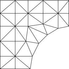
The ﬁnite element method (FEM) is a special case of the Rayleigh–Ritz method. In the FEM the subspace S and in particular the basis {φi} is chosen in a particularly clever way. For simplicity we assume that the domain Ω is a simply connected domain with a polygonal boundary, c.f. Fig 1.5. (This means that the boundary is composed entirely of straight line segments.) This domain is now partitioned into triangular subdomains

Finite element spaces for solving (1.40)–(1.42) are typically composed of functions that are continuous in Ω and are polynomials on the individual subdomains Te. Such functions are called piecewise polynomials. Notice that this construction provides a subspace of the Hilbert space H but not of V , i.e., the functions in the ﬁnite element space are not very smooth and the natural boundary conditions are not satisﬁed.

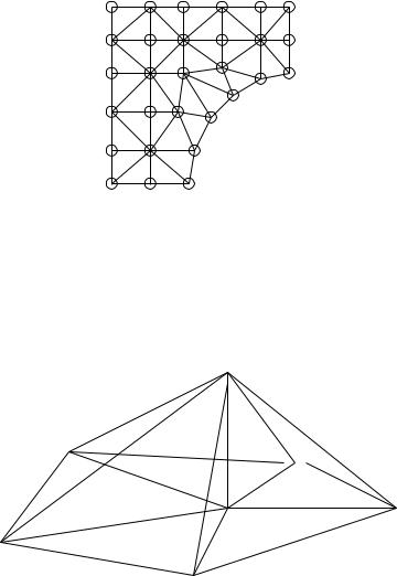
An essential issue is the selection of the basis of the ﬁnite element space S. If S1 H is the space of continuous, piecewise linear functions (the restriction to Te is a polynomial of degree 1) then a function in S1 is uniquely determined by its values at the vertices of the triangles. Let these nodes, except those on the boundary portion C1, be numbered from 1 to n, see Fig. 1.6. Let the coordinates of the i-th node be (xi, yi). Then φi(x, y) S1 is deﬁned by

1.6. THE 2D LAPLACE EIGENVALUE PROBLEM

17	20	24	27	29
16				29
15	19	23	26	28
13				28
11	14	21
11	14
10
7	9		22	25
	9		22
			18
6			18
6
4		12
4
3		8
		8
1		5
2

Figure 1.6: Numbering of nodes on Ω (piecewise linear polynomials)

(1.65)	φi((xj , yj )) := δij =	1	i = j
		0	i 6= j

A typical basis function φi is sketched in Figure 1.7.

Figure 1.7: A piecewise linear basis function (or hat function)

Another often used ﬁnite element element space is S2 H, the space of continuous, piecewise quadratic polynomials. These functions are (or can be) uniquely determined by their values at the vertices and edge midpoints of the triangle. The basis functions are deﬁned according to (1.65). There are two kinds of basis functions φi now, ﬁrst those that are 1 at a vertex and second those that are 1 in an edge midpoint, cf. Fig. 1.8. One immediately sees that for most i 6= j

(1.66) a(φi, φj ) = 0, (φi, φj ) = 0.

Therefore the matrices A and M in (1.62) will be sparse. The matrix M is positive deﬁnite as

	N	N								N
	X	X								X
(1.67)	xT Mx =	xixj mij =	xixj (φi, φj ) = (u, u) > 0, u =							xiφi 6= 0,
	i,j=1	i,j=1								i=1
				\|\|		\|\|
because the φ are linearly independent and because					u		=		(u, u) is a norm. Similarly
it is shown thati								p

xT Ax ≥ 0.

<<< < Предыдущая 1 2 3 45 / 635 6 7 8 9 10 11 12 13 14 15 16 17 18 19 20 21 22 23 24 25 > Следующая >>>

Соседние файлы в предмете [НЕСОРТИРОВАННОЕ]

#
09.02.20151.89 Mб26lection_part1-2.pdf
#
09.02.20152.93 Mб20lection_part3.pdf
#
22.03.20163.28 Mб7Lecture 02.pdf
#
22.03.20162.59 Mб6Lecture 07.pdf
#
22.03.201613.56 Кб8lecture marketing.docx
#
22.03.20162.32 Mб45Lecture Notes on Solving Large Scale Eigenvalue Problems.pdf
#
22.03.20163.59 Mб6Lecture_01.pdf
#
22.03.20163.16 Mб8Lecture_06.pdf
#
22.03.20162.32 Mб9Lecture_09.pdf
#
22.03.20163.22 Mб6Lecture_10.pdf
#
22.03.20163.08 Mб8Lecture_11_1.pdf

17	20	24	27	29
16				29
15	19	23	26	28
13				28
11	14	21
11	14
10
7	9		22	25
	9		22
			18
6			18
6
4		12
4
3		8
		8
1		5
2

17	20	24	27	29
16				29
15	19	23	26	28
13				28
11	14	21
11	14
10
7	9		22	25
	9		22
			18
6			18
6
4		12
4
3		8
		8
1		5
2

17	20	24	27	29
16				29
15	19	23	26	28
13				28
11	14	21
11	14
10
7	9		22	25
	9		22
			18
6			18
6
4		12
4
3		8
		8
1		5
2