

Lect5-Optical_fibers_2
.pdfDispersion-Compensating Fiber
The DCF needed to compensate for 1700 ps with a large negative-dispersion parameter
i.e. we need Tchrom + |
TDCF = 0 |
TDCF |
= DDCF(λ) Δλ LDCF |
suppose typical ratio of L/LDCF ~ 6 – 7, we assume LDCF = 15 km |
|
=>DDCF(λ) ~ -113 ps/(km-nm) |
|
*Typically, only one wavelength can be compensated exactly. |
|
Better CD compensation requires both dispersion and dispersion |
|
slope compensation. |
121 |

Dispersion slope compensation
Compensating the dispersion slope produces the additional requirement:
L2 dD2/dλ = - L1 dD1/dλ
The compensating fiber must have a negative dispersion slope, and that the dispersion and slope values need to be compensated for a given length.
D2 L2 = - D1 L1
L2 dD2/dλ = - L1 dD1/dλ
=> Dispersion and slope compensation: D2 / (dD2/dλ) = D1 / (dD1/dλ)
(In practice, two fibers are used, one of which has negative slope, in which the pulse
wavelength is at zero-dispersion wavelength λzD.)
122
Dispersion slope compensation
km] |
|
|
|
|
|
|
|
|
|
|
|
|
|
[ps/nm- |
|
|
16 |
17 18 |
+ve |
|
|
|
|
||||
Dispersion |
|
|
SM fiber |
|
|
|
|
|
-96 |
-ve (due to large -ve Dwg) |
|||
|
|
|
λ1 |
λ2 |
|
λ |
|
|
|
DCF |
|
|
|
|
|
|
-102 |
|
|
|
|
|
|
|
|||
|
|
|
|
-108 |
|
|
Within the spectral window (λ1, λ2), DDCF/DSM = -6 |
||||||
SDCF = |
-12/(λ2 – λ1); SSM = |
2/(λ2 – λ1) |
=> SDCF/SSM = -6 |
|||
=> Dispersion slope compensation: (DSM/SSM) / (DDCF/SDCF) = 1 123
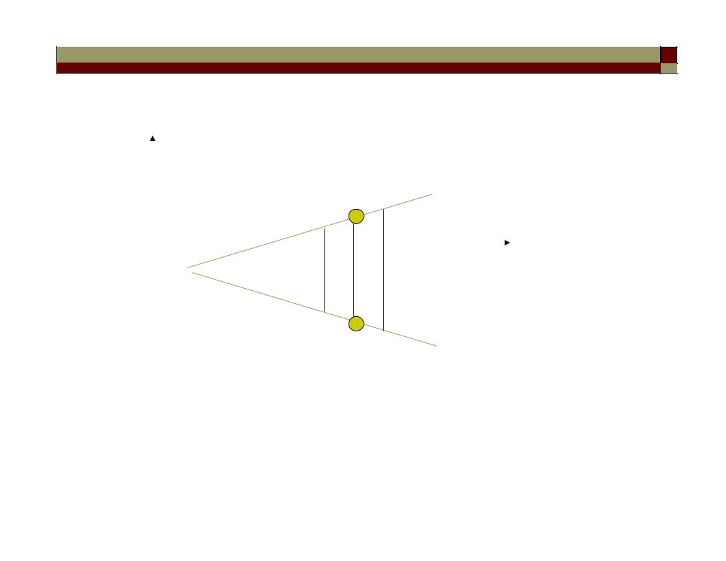
Disadvantages in using DCF
• Added loss associated with the increased fiber span
• Nonlinear optic effects may degrade the signal over the long length of the fiber if the signal is of sufficient intensity.
• Links that use DCF often require an amplifier stage to compensate the added loss.
-D |
g |
-D |
g |
Splice loss |
Long DCF (loss, possible nonlinear optic effects) |
124
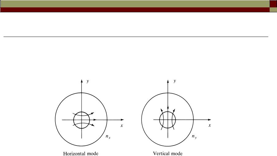
Polarization Mode Dispersion (PMD)
• In a single-mode optical fiber, the optical signal is carried by the linearly polarized “fundamental mode” LP01, which has
two polarization components that are orthogonal.
(note that x and y
are chosen arbitrarily)
• In a real fiber (i.e. ngx ≠ ngy), the two orthogonal polarization modes propagate at different group velocities, resulting in pulse broadening – polarization mode dispersion.
125
Polarization Mode Dispersion (PMD)
Ey |
|
|
Ey |
|
|
T |
|
||
|
|
|
|
||||||
|
|
|
|
|
|
|
|
|
|
|
|
|
|
|
vgy = c/ngy |
|
|
|
|
|
|
|
|
|
|
|
|
|
|
|
|
|
|
|
|
|
|
|
|
|
|
|
|
||
|
|
|
|
|
|
|
|
|
|
|
|
|
|
|
|||
Ex |
|
|
|
|
vgx = c/ngx ≠ vgy |
Ex |
|
|
|
|
|
|
|
|
t |
|
|
|
|
|
|
|
|
|
|
|
|
|
|
||||||
|
|
|
|
|
|
|
|
|
|
|
|
|
|||||
|
|
|
|
|
|
|
|
|
|||||||||
|
|
|
|
t |
|
|
|
|
|
|
|
|
|||||
|
|
|
|
|
|
|
|
|
|
|
|
|
|
|
|
||
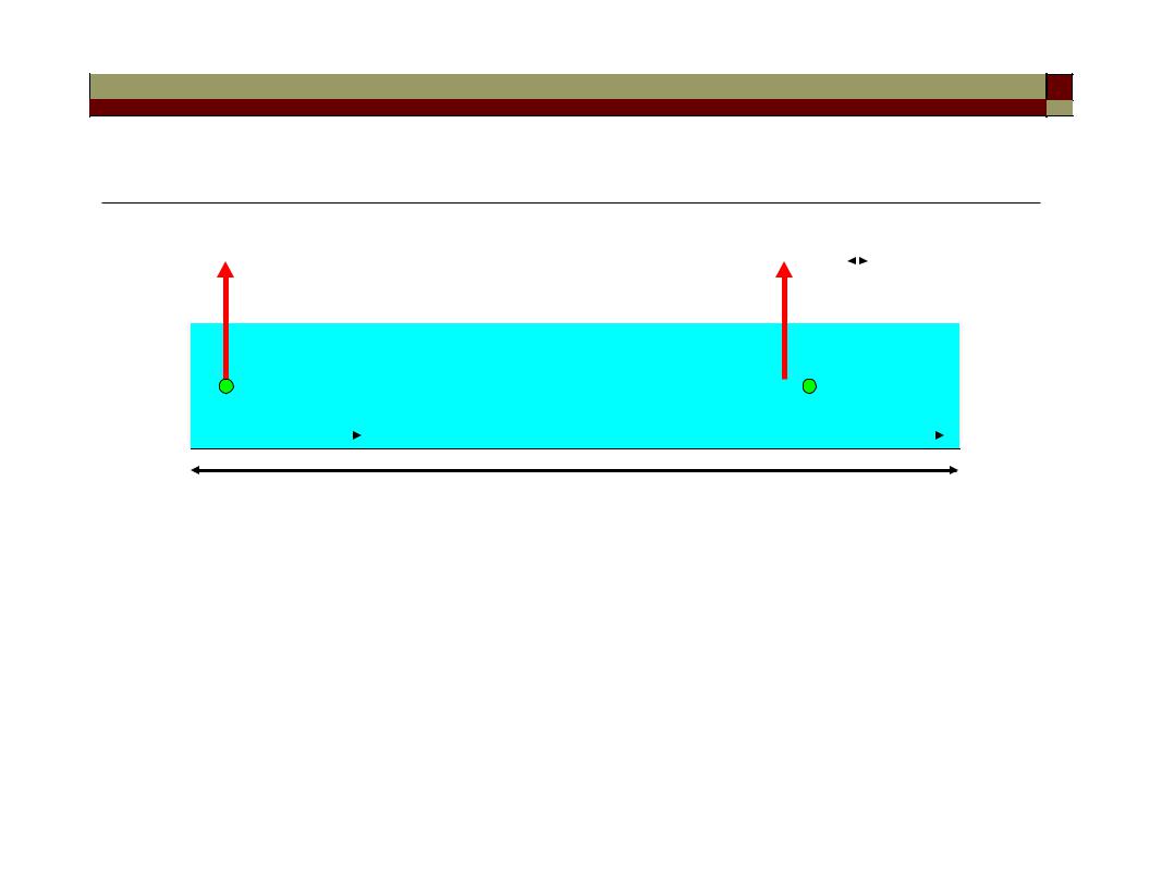
Single-mode fiber L km
1.Pulse broadening due to the orthogonal polarization modes (The time delay between the two polarization components is characterized as the differential group delay (DGD).)
2.Polarization varies along the fiber length
126

Polarization Mode Dispersion (PMD)
• The refractive index difference is known as birefringence.
B = nx - ny |
(~ 10-6 - 10-5 for |
|
single-mode fibers) |
assuming nx > ny => y is the fast axis, x is the slow axis.
*B varies randomly because of thermal and mechanical stresses over time (due to randomly varying environmental factors in submarine, terrestrial, aerial, and buried fiber cables).
=> PMD is a statistical process !
127
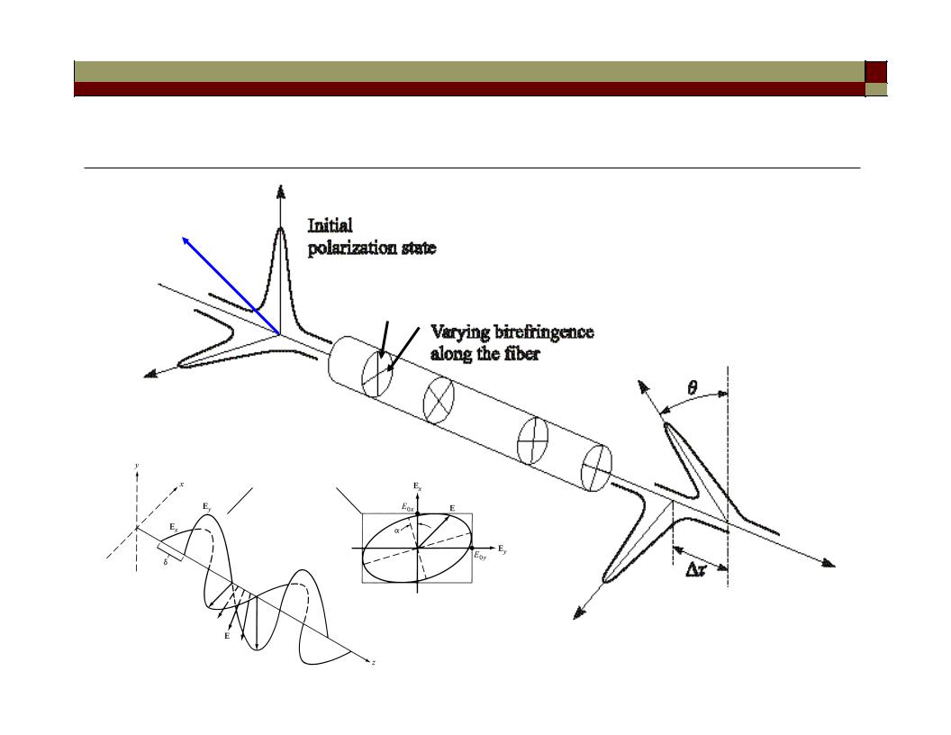
Randomly varying birefringence along the fiber
y
E
Principal axes
x
Elliptical polarization
128

Randomly varying birefringence along the fiber
• The polarization state of light propagating in fibers with randomly varying birefringence will generally be elliptical and would quickly reach a state of arbitrary polarization.
*However, the final polarization state is not of concern for most lightwave systems as photodetectors are insensitive to the state of polarization.
(Note: the recent revival of technology developments in “Coherent Optical Communications” do require polarization state to be analyzed!)
• A simple model of PMD divides the fiber into a large number of segments. Both the magnitude of birefringence B and the orientation of the principal axes remain constant in each section but changes
randomly from section to section.
129
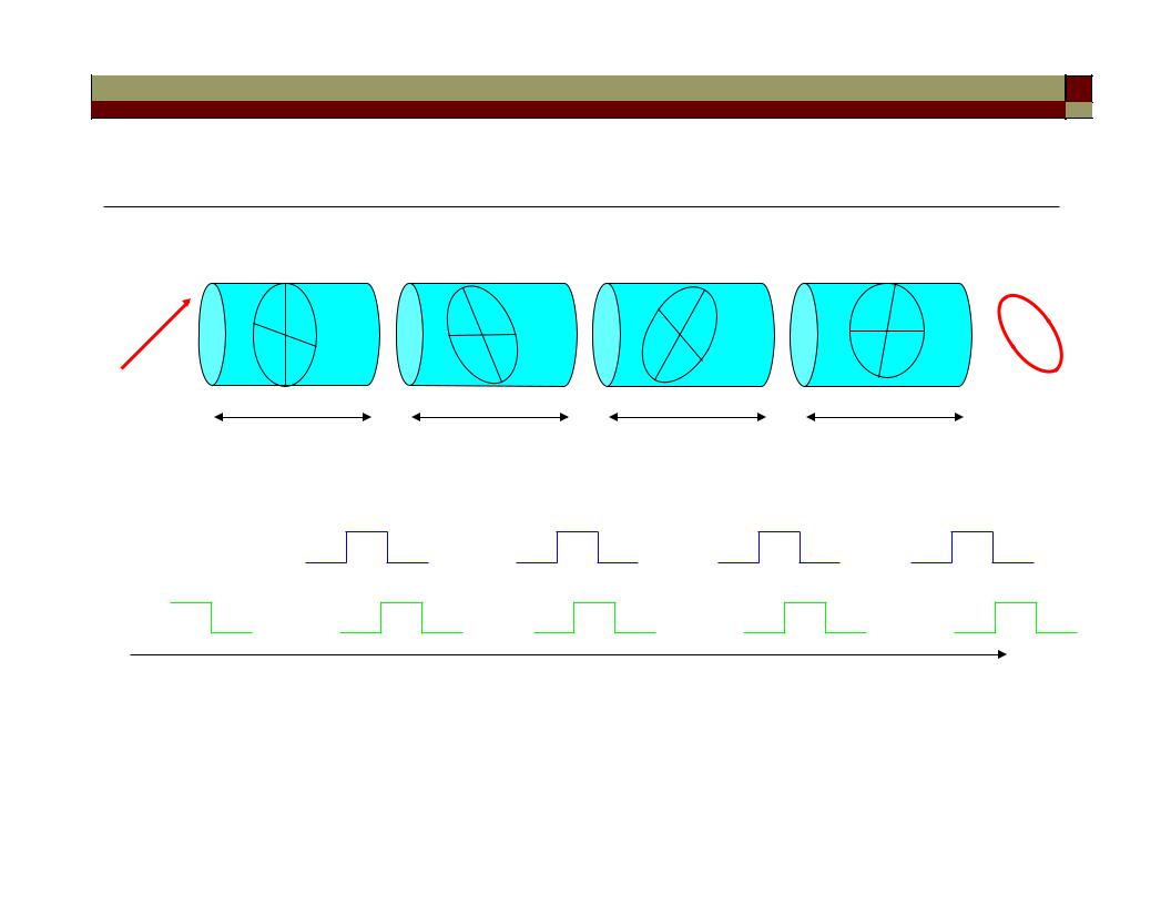
A simple model of PMD
B0 |
B1 |
B2 |
B3 |
Lo |
L1 |
L2 |
L3 |
Ex 

Ey 
t
Randomly changing differential group delay (DGD)
130