

Excel2010
.pdfExample 5.38
In order to improve the Excel document that you have given to your math teacher, now, you can prepare another formula, which defines the letter grades for students. If the average of a student is lower than 60, it will write ‘F’ and so on. Your teacher has provided the Letter Grade conversion table in the range J3:K9.
Figure 5.33: Calculating letter grades
Analysis and Solution:
You can use both; HLookUp or VLookUp, according to your worksheet design. But, if you design the worksheet as in Figure 5.33, because the values that you search are located in the left most column, you need to use VLookUp.
When looking up the letter grade of the first student,
you’ll write the formula in F3
referring to the average in E3.
The table is in J3:K9 and you want
the VLookUp function to return the value in the second column as the result. The formula for the first student becomes
=VLookUp(E3, J3:K9,2,TRUE)
Because you don’t change the address of Letter Grade Table (J3:K9) for every student, this is an absolute address. As you know from previous sections, you place a ‘$’ sign to the front of an absolute address;
$J$3:$K$9.
Because the Lookup value cell changes for every student, it is a relative address. Finally the formula becomes
=VLookUp(E3, $J$3:$K$9, 2, TRUE)
The formula is ready and can be copied for other students.
Functions and Formulas |
91 |
Data Data
Apples Lemons
Bananas Pears
|
A |
B |
|
1 |
Product |
Count |
|
2 |
Bananas |
25 |
|
3 |
Oranges |
38 |
|
4 |
Apples |
40 |
|
5 |
Pears |
41 |
|
6 |
|
|
|
7 |
Find in the |
Oranges |
|
8 |
List |
2 |
|
|
|
|
|
|
|
|
|
Figure 5.34: Using Defined Names
5.5.6.3 Index()
Index and Match functions (instead of vlookup) can be used in collaboration to return values from tables. Index function returns a value (or the reference to a value) from/within a range. Match function Returns the relative position of an item in a range that matches a specified value in a specified order.
Usage: INDEX(array, row_num, [column_num])
Example 5.39
=INDEX(A2:B3,2,2) Value at the intersection of the 2nd row and 2nd column in the range (Pears)
=INDEX(A2:B3,2,1) Value at the intersection of the 2nd row and 1st column in the range (Bananas)
5.5.6.4 Match()
MATCH function can be used instead of the LOOKUP functions when you need the position of an item in a range instead of the item itself. It returns the relative position of an item in an array that matches a specified value in a specified order.
Example 5.40
According to table next, find the position of the item specified in the cell B7 (Oranges).
Product list is in A2:A5. The item that we are searching for is in B7. And match type is 0 (zero), because we search for an exact match.
Finally we write the formula in B8
=MATCH(B7,A2:A5,0)
And it will return 2, because Oranges is in the second cell in our search range.
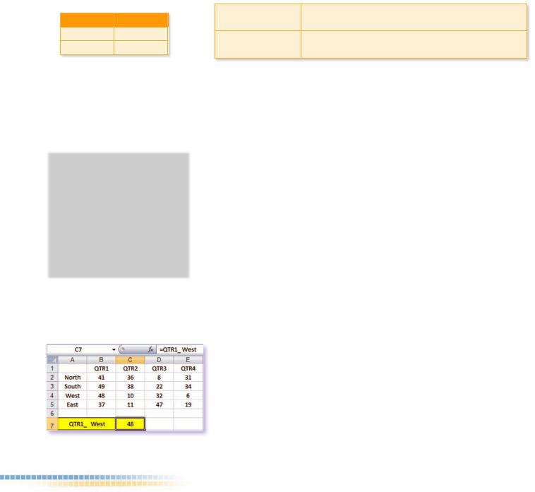
5.5.6.5 Using Defined Names
There is another method to dereference two way lookups: using Defined names. You provide a name for each row and column of the table. A quick way to do this is to select the table and choose Formulas Defined NamesCreate From Selection.
In the ‘Create Names from Selection’ dialog box, select the ‘Top Row’ and ‘Left Column’ check boxes. After creating the names, you can use a simple formula, such as:
Example 5.41
QTR1_ is the name of the range B2:B5. West is the name of the range B4:E4. Then the formula
=QTR1_ West
will give the intersection of these ranges (48)
92 |
Microsoft Excel |

5.5.7 Database Functions
For a good analysis of data, you need to have a well organized data list. This is called a database. Microsoft Excel provides a flexible environment for you to prepare well organized lists and powerful functions to process and decide fast. For this purpose, it includes many functions that analyze data stored in lists or databases. One of these functions, referred to collectively as the Dfunctions, uses three arguments: database, field, and criteria. These arguments refer to the worksheet ranges that are used by the function. When placing criteria:
Take care that your criteria field does not overlap with your database.
Do not place your criteria field beneath your database.
Example 5.42
The Assistant director of Atlanta High School is using an Excel worksheet to keep track of students attendance. In his form, he has 6 columns of information; Class, Name, Date, Subject, Hours, and Motivation. But, because it’s quite difficult to count or to filter and then process all the data, he wants a formula that counts automatically all the data with the given criteria. In the example below, he wants to search all data for Todd Rafferty’s unmotivated absences. (Design all the data in a worksheet and write your formula using the DSum function).
CRITERIA
Class |
Name |
Date |
|
Lesson |
Hours |
Motivated |
|
Todd Rafferty |
|
|
|
|
FALSE |
|
|
RESULT |
|
|
|
|
|
|
4 |
|
|
|
|
|
|
DATABASE |
|
|
|
|
|
|
|
|
|
|
|
Class |
Name |
Date |
|
Lesson |
Hours |
Motivated |
11A |
David Shadovitz |
2/17/2003 |
|
Maths |
2 |
TRUE |
11A |
Todd Rafferty |
2/17/2004 |
|
Maths |
2 |
FALSE |
11A |
Pablo Varando |
2/18/2004 |
|
Chemistry |
2 |
TRUE |
11A |
Brendan Hara |
2/19/2004 |
|
Informatics |
2 |
TRUE |
11A |
Pete Thomas |
2/20/2004 |
|
Informatics |
2 |
FALSE |
11A |
Todd Rafferty |
2/21/2004 |
|
Physics |
1 |
TRUE |
11A |
Todd Rafferty |
2/24/2004 |
|
Physics |
2 |
FALSE |
11A |
Simon Horwith |
2/25/2004 |
|
Physics |
1 |
TRUE |
11A |
David Shadovitz |
2/26/2004 |
|
Physics |
2 |
TRUE |
11A |
David Shadovitz |
2/27/2004 |
|
Chemistry |
2 |
FALSE |
|
|
|
|
|
|
|
Functions and Formulas |
93 |
|
|
|
|

Analysis and Solution:
As it is explained in the question, we need six fields: Class, Name and Surname, Date of absence, Subject, Number of hours, and if the absence is Motivated or not. (Motivated “True” means the student has permission.)
Because the database might grow bigger, the criteria field should not be beneath the database. So, we can place it to the top of the sheet starting from B2 till the end of G3 that includes your search values together with the titles.
Every time we add another absence, we’ll add to the bottom of the database and it will grow bigger. We’ll use the DSum function which adds the numbers in the field column of records in the database that match the criteria.
=DSum (Database, Field, Criteria)
We want the result to appear in the 5th row, so we will write the formula into the cell B5. The Database range according to the given table is B7:G18, where B7 is the start address of the Database. But, because your table will grow bigger, you shouldn’t use G18 as the Last cell. Rather than 18, you should use something big enough to handle your future table; like 2000. And, the Criteria range is B2:G3 and we want the Hours field to be summed according to the Criteria. Then, the formula becomes;
=DSum(B7:G2000,"Hours",B2:G3)
It will calculate the sum of the numbers in the Hours column with the records complying with the criteria described in the Criteria range. When you enter a name in the criteria name part, all the absences with that name will be processed. If you want to see the total unmotivated absence of this student, in the motivation field, write FALSE. Or, if you want absences from a specific subject then write also the subject name. The function will return the sum of the Hours column with the records satisfying your criteria.
94 |
Microsoft Excel |

Questions
1. If cell A5 contains a formula which |
|
A |
|
produces 25, what can be the |
|
|
|
1 |
10 |
||
formula in A5? |
|||
2 |
20 |
||
|
|||
a. =Sum (A1:A4) |
3 |
30 |
|
b. =Min (A1:A4) |
4 |
40 |
|
c. =Average (A1:A4) |
5 |
? |
|
|
|
||
d. =Count (A1:A4) |
|
|
2.According to the figure in question 1, if the value of A5 is 40, what can be the formula in it?
a. =Count (A1:A4) |
b. =Sum (A1:A4) |
c. =Average (A1:A4) |
d. =Max (A1:A4) |
3.If you want to type a formula in a cell, you must start your formula with a ..... sign.
a. = |
b. ! |
c. $ |
d. ? |
4.Which of the followings is not a Microsoft Excel function?
a. If |
b. List |
c. Max |
|
d. Count |
|
5. Look at the next figure. The |
|
|
|||
|
A |
||||
A5 |
cell contains |
the |
|
|
|
1 |
10 |
||||
formula =A1+A2+A3. |
|||||
2 |
20 |
||||
|
|
|
|||
What can be the reason for |
3 |
January |
|||
the error message #VALUE!? |
4 |
|
|||
a. The column is too narrow |
5 |
#VALUE! |
|||
b.A3 contains text
c.One of the columns is deleted
d.Formula is misspelled
6. What is the result |
|
A |
B |
C |
D |
||
of the |
function |
|
|
|
|
|
|
1 |
100 |
12 |
128 |
20 |
|||
=Max(B1:D4) |
|||||||
2 |
200 |
22 |
601 |
60 |
|||
|
|
||||||
|
|
3 |
400 |
68 |
288 |
80 |
|
|
|
4 |
800 |
21 |
204 |
97 |
|
a. 800 |
b. 68 |
|
c. 601 |
d. 288 |
|||
7.Which function returns the result of the mathematical expression Sin(30)?
a.=Sin(30)
b.=Sin(30*P/180)
c.=Sin(30*180/Pi())
d.=Sin(30*Pi()/180)
8.What is the result of the formula in A4?
|
|
A |
|
B |
|
C |
|
|
1 |
5 |
|
2 |
|
|
|
|
2 |
5 |
|
3 |
|
|
|
|
3 |
1 |
|
7 |
|
|
|
|
4 |
=AVERAGE(A2:B3)+SUM(A2:B3) |
|
||||
|
|
|
|
|
|
|
|
a. 26,8 |
b. 3,8 |
c. 16 |
d. 20 |
||||
9.The result of =Int(-1.5) is less than the result of=Trunc(-1.5)
TRUE |
FALSE |
Functions and Formulas |
95 |

10.According to the formulas in C1 and C2, which one is true?
A |
B |
C |
1 John |
3 =If(B1<=2,"Very bad" ,If(B1<4, "Bad", "Perfect")) |
|
2 Smith 4 =If(B2<=2,"Very bad" ,If(B2<4,"Bad","Perfect"))
a.John : Very bad Smith : Bad
b.John : Bad Smith : Bad
c.John : Very bad Smith : Very bad
d.John : Bad Smith : Perfect
11.Which formula must be written into cell B2 to calculate the volume of the cube in the figure?
AB
1 A: |
4 |
2 Volume: 64
a. = B1*B1*B1
c. = A1*A1*A1
A A
A
b. = B2*B2*B2
d. = Cube(B1)
12.Find the result of the formula =VLookUp (2, A2:D4, 3)
|
|
A |
B |
C |
D |
|
|
1 |
Id |
Name |
Surname 1st Term |
|
|
|
2 |
1 |
Andrew |
Jackson |
3 |
|
|
3 |
2 |
Thomas |
Ericsson |
4 |
|
|
4 |
3 |
Laura |
Callahan |
5 |
|
a. 2 |
b. Andrew |
c. Ericsson |
d. 4 |
|||
13.What is the result of the formula =Int(3.741696) + Round(36.9245,2)
a. 40,1 |
b. 40 |
c. 39,92 |
d. 39 |
14.Match the following functions with the definitions?
Functions |
|
Definitions |
Min |
|
Calculates the average value of a list of numbers |
|
|
|
Max |
|
Adds a list of numbers. |
|
|
|
Average |
|
Finds the smallest value in a list of numbers. |
|
|
|
Sum |
|
Finds the largest value in a list of numbers. |
|
|
|
15. 
In cells B1 through G1 these values are entered arbitrarily. What is the result of the formula =CountIf(B1:G1, “>5”)
a. 0 |
b. 7 |
c. 1 |
d. 2 |
16.The LookUp functions allow you to
a.Retrieve the names of workbooks and worksheets.
b.Retrieve information according to given criteria.
c.Dynamically change information in different workbooks and worksheets.
d.Retrieve information stored in different reseources.
Project
1.According to the figure next write the necessary formulas to
calculate the average salary of all employees
find the maximum salary
find the minimum salary
find the total salary
A |
B |
C |
1Tree Star Trade Company
2 |
Employee |
|
City |
Salary |
3 |
Selena Bainum |
|
Berlin |
$ 1520 |
4 |
Raymond Camden |
|
Mexico |
$ 2500 |
5 |
Paul Hastings |
|
Moscow |
$ 1800 |
6 |
Kevin Schmidt |
|
London |
$ 3200 |
7 |
Pete Thomas |
|
Istanbul |
$ 5210 |
8 |
Nicholas Tunney |
|
Madrid |
$ 850 |
9 |
|
|
|
|
10 The Average salary of all |
employees : |
? |
||
11 |
Maximum salary : |
|
? |
|
12 |
Minimum salary : |
|
? |
|
13 |
Total salary : |
|
? |
|
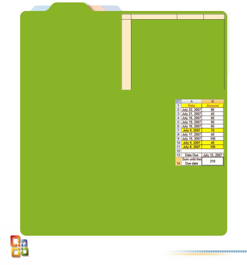
2.Your father is running a small business. Some companies buy some products and they give some checks. Your father stores due dates and amounts of these checks in a worksheet.
When he has to pay cash, he uses the same worksheet to see if the amount of money that he is going to collect is enough or not.
Write a function in B14, so that, it will take the Sum of the Amounts (B2:B11), if the date in column B is less than the Due Date (B13).
3.In the following Figure, write a formula
in A3 to calculate the multiplication of the numbers in range A1:F1.
in B6 to calculate the absolute value of the given number in A6.
in D6 to calculate the square-root of the given number in C6.
in F7 to calculate xy
|
A |
|
B |
C |
D |
E |
F |
1 |
6 |
|
7 |
8 |
9 |
10 |
11 |
2 |
|
Write the multiplication of the numbers above using |
|||||
|
|
|
“product” function. |
|
|||
|
|
|
|
|
|||
3 |
|
|
|
|
Formula |
|
|
4 |
|
|
|
|
|
|
|
5 |
x |
|
ABS |
Y |
SQRT |
Enter base (X) |
2 |
6 |
-8 |
|
Formula |
256 |
Formula |
Enter power (Y) |
3 |
7 |
|
|
|
|
|
XY |
Formula |
Functions and Formulas |
97 |
4. In an apartment building, you have 5 floors and 5 |
|
A |
B |
C |
|
different entrances. On each floor, there are three |
1 |
Apartment # |
Entrance # |
Floor # |
|
2 |
43 |
? |
? |
||
apartments. Write a formula that will take an |
|||||
|
|
|
|
apartment number from cell A2 and show the floor and entrance numbers in cells B2 and C2.
5. Create a mini trigonometric table below.
|
A |
B |
C |
D |
E |
1 |
|
Mini |
Trigonometric |
Table |
|
2 |
Degree |
Radian |
Sinus |
Cosine |
Tangent |
|
|
|
|
|
|
30
410
520
630
740
850
960
1070
1180
1290
6.Use the following functions on the table below.
|
A |
B |
C |
D |
E |
F |
1 |
ID |
Students |
Grades |
Int |
Round |
Trunc |
2 |
1 |
Raymond Camden |
2.460 |
? |
? |
? |
3 |
2 |
Paul Hastings |
3.689 |
|
|
|
4 |
3 |
Kevin Schmidt |
3.840 |
|
|
|
5 |
4 |
Pete Thomas |
3.118 |
|
|
|
6 |
5 |
Nicholas Tunney |
2.060 |
|
|
|
7. Write a formula which can calculate the total salary of the employees in the city given by cell C2.
|
A |
B |
C |
D |
|
1 |
Id |
Employee |
City |
Salary |
|
2 |
|
|
London |
|
|
3Total salary of employees live in given city?
4 |
1 |
Kevin Schmidt |
New York |
400 |
5 |
2 |
David `Shadovitz |
London |
400 |
6 |
3 |
Pete Thomas |
London |
400 |
7 |
4 |
Nicholas Tunney |
New York |
350 |
8 |
5 |
Kevin Schmidt |
London |
400 |
9 |
6 |
David Shadovitz |
New York |
615 |
10 |
7 |
Pete Thomas |
London |
540 |
11 |
8 |
Nicholas Tunney |
London |
1000 |

8. Draw the following chart using Sin and Cos functions.
9. Write the necessary formula, |
|
|
A |
B |
C |
D |
E |
|
in column B to show |
the |
1 |
Name & Surname |
Length |
Space |
Name |
Surname |
|
lengths of adjacent names in |
2 |
Samuel Neff |
11 |
|
Samuel |
Neff |
||
3 |
Brendan Hara |
12 |
|
Brendan |
Hara |
|||
column A. |
|
|
||||||
|
4 |
Jeremy Petersen |
15 |
|
Jeremy |
Petersen |
||
using Find, Left, Mid and Len |
|
|||||||
5 |
Todd Rafferty |
13 |
|
Todd |
Rafferty |
|||
functions |
to separate |
the |
6 |
Kevin Schmidt |
13 |
|
Kevin |
Schmidt |
texts in |
column A to |
the |
7 |
David Shadovitz |
15 |
|
David |
Shadovitz |
columns D and E as shown |
8 |
Pete Thomas |
11 |
|
Pete |
Thomas |
||
in the figure. |
|
9 |
Nicholas Tunney |
15 |
|
Nicholas |
Tunney |
|
|
|
|
|
|
|
|
||
10. Write the necessary formulas |
|
A |
B |
C |
D |
E |
|
F |
G |
into the cells between B11 |
1 |
|
|
EXAMINATION RESULTS |
|
|
|||
through G11 that will accept C9 |
2 |
Id |
Name |
Surname |
Maths |
Physics |
|
chemistry |
AVERAGE |
as student id using the |
3 |
1 |
Samuel |
Neff |
5 |
5 |
|
5 |
5 |
“VLookUp” function. |
4 |
2 |
Brendan |
Hara |
3 |
2 |
|
4 |
3 |
5 |
3 |
Jeremy |
Peterson |
2 |
4 |
|
3 |
3 |
|
|
|
||||||||
|
6 |
4 |
Todd |
Rafferty |
4 |
5 |
|
3 |
4 |
|
7 |
5 |
Kevin |
Schmidt |
3 |
4 |
|
5 |
4 |
|
8 |
|
|
|
|
|
|
|
|
|
9 |
|
Enter Id: |
4 |
|
|
|
|
|
|
10 |
|
Name |
Surname |
Maths |
Physics |
|
chemistry |
AVERAGE |
|
11 |
|
Todd |
Rafferty |
4 |
5 |
|
3 |
4 |
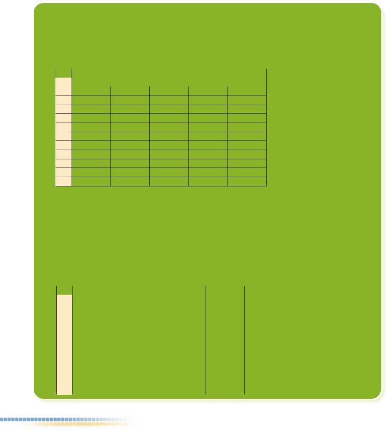
11.Write the necessary formulas into range C9:C12 that will read the class name from C7 and show the requested class list in the cells.
|
A |
B |
C |
D |
E |
1 |
|
11A |
11B |
11C |
11D |
2 |
Index |
Name and |
Name and |
Name and |
Name and |
|
|
surname |
surname |
surname |
surname |
3 |
1 |
Simon harwith |
Pete Thomas |
Selene Bainum |
Hanna Moos |
4 |
2 |
Stephen Milligan |
Nicholas Tunney |
Geoff Bowers |
Bab Hanks |
5 |
3 |
Samuel Neff |
Jochem Dieten |
Rob Brooks |
Martin Sammer |
6 |
4 |
David Shadavitz |
Pablo Varanda |
Raymond Camden |
Victoria Ashworth |
7 |
|
Enter Class: |
11C |
|
|
8 |
|
Index |
Name and |
|
|
|
surname |
|
|
||
|
|
|
|
|
|
9 |
|
1 |
Selene Bainum |
|
|
10 |
|
2 |
Geoff Bowers |
|
|
11 |
|
3 |
Rob Brooks |
|
|
12 |
|
4 |
Raymond Camden |
|
|
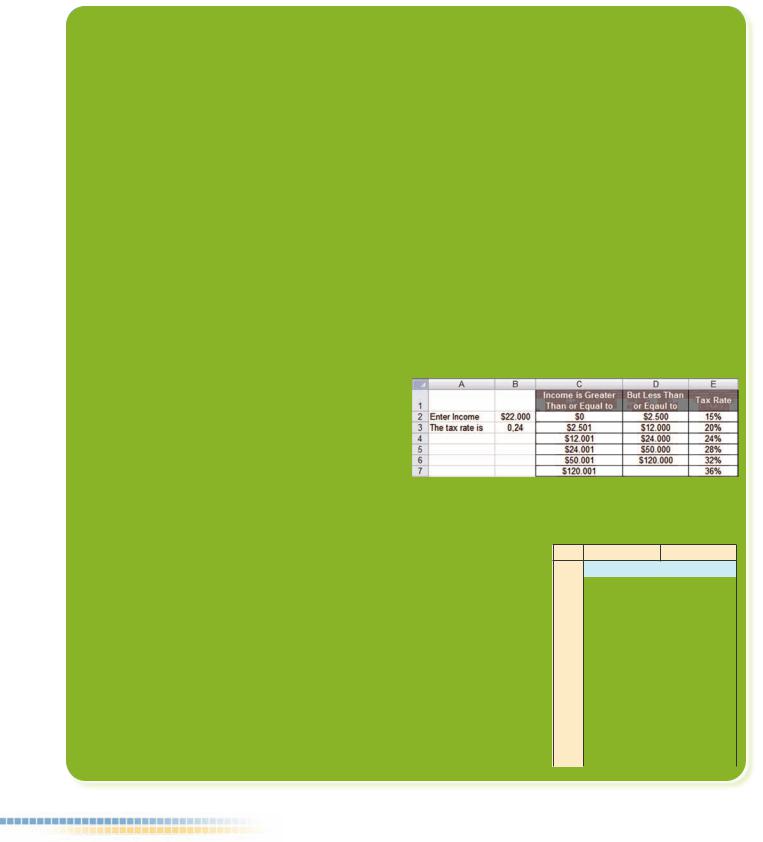
12.A very common use for a lookup formula involves an income tax rate schedule (see the figure next). The tax rate schedule shows the income tax rates for various income levels.
Write the necessary formula to the B3 cell that checks the income level (B2) and returns the Tax rate.
13.In exchange offices, everyday, money from many different currencies are exchanged. Because they are afraid of making mistakes, they decided to have an exchange program. In this document, the first part will have a table of conversion from all other currencies into a base one. (In this figure, the base currency is TL.) They want to write exchange currencies in cells A12 and B12. When they write the amount of the first currency into A13, they want to see the converted value in B13.
AB
1EXCHANGE RATES
2 |
Currencles |
TL |
3 |
Dollar |
1.38 |
4 |
Euro |
1.82 |
5 |
TL |
1 |
6 |
Pound |
2.57 |
7 |
Ruble |
0.47 |
8 |
Yen |
1.5 |
9 |
Dinar |
1.3 |
10 |
|
|
11 |
From |
To |
12 |
Dollar |
Euro |
13 |
10 |
7.58 |