1.5. Measures of dispersion for ungrouped data

In statistics, in order to describe the data set accurately statisticians must know more than measures of central tendency. Two data sets with the same mean may have completely different spreads. The variation among values of observations for one data set may be much larger or smaller than for the other data set.

Remark:

The words dispersion, spread, and variation have the same meaning.

Example:

Consider the following two samples:

Sample1: 66, 66, 66, 67, 67, 67, 68, 69

Sample2: 43, 44, 50, 54, 67, 90, 91, 97

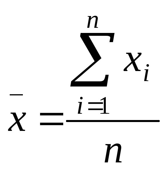
The mean of sample1 is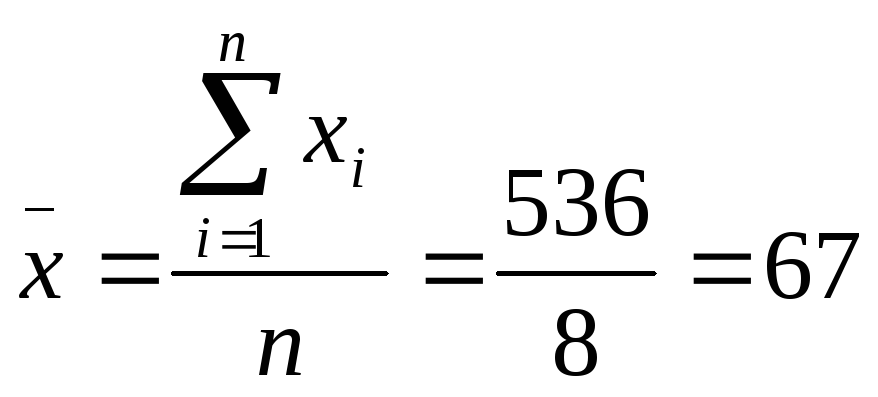

The mean of sample2 is .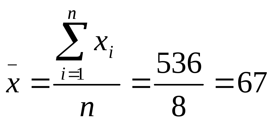

Each of these samples has a mean equal to 67. However, the dispersion of the observations in the two samples differs greatly. In the first sample all observations are grouped within 2 units of the mean. Only one observation (67) is closer than 13 units to the mean of the second sample, and some are as far away as 30 units. Thus, the mean, median, or mode is usually not by itself a sufficient measure to reveal the shape of the distribution of a data set. We also need a measure that can provide some information about the variation among data values. The measures that help us to know about the spread of data set are called the measures of dispersion. The measures of central tendency and dispersion taken together give a better picture of a data set than measure of central tendency alone. Several quantities that are used as measures of dispersion are the range, the mean absolute deviation, the variance, and the standard deviation.

1.5.1. Range

The simplest measure of variability for a set of data is the range.

Definition:

The range for a set of data is the difference between the largest and smallest values in the set.

Range=Largest value-Smallest value

Example:

Find the range for the sample observations

13, 23, 11, 17, 25, 18, 14, 24

Solution:

We see that the largest observation is 25 and the smallest observation

is 11. The range is 25-11=14.

Example:

A sample is composed of the observations

67, 79, 87, 97, 93, 57, 44, 80, 47, 78, 81, 90, 88, 91

Find the range.

Solution:

The largest observation is 97; the smallest observation is 44.

The range is .

1.5.2. The mean absolute deviation

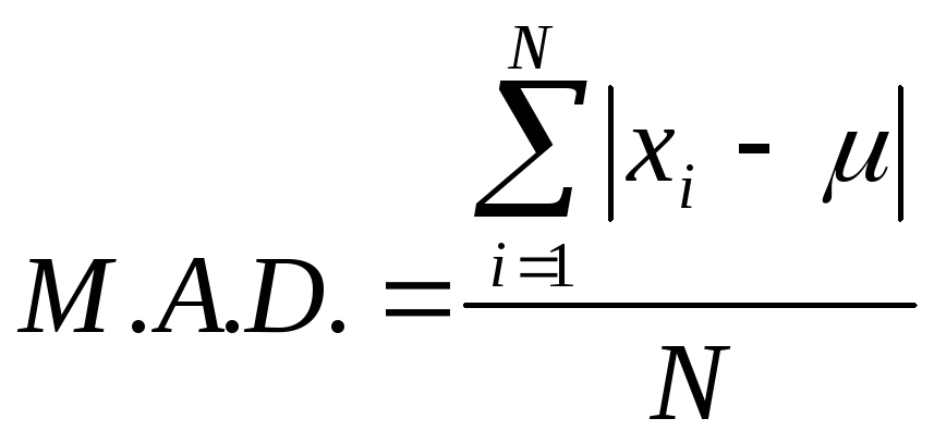
The mean absolute deviation is defined exactly as the words indicate. The word “deviation” refers to the deviation of each member from the mean of the population. The term “absolute deviation” means the numerical (i.e. positive) value of the deviation, and the “mean absolute deviation” is simply the arithmetic mean of the absolute deviations.

Let denote the members of a population, whose mean is. Their mean absolute deviation, denoted by is

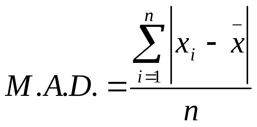
For the sample of observations, with mean, mean absolute deviation is defined analogously

To calculate mean absolute deviation it is necessary to take following steps:

1. Find (or)

2. Find and record the signed differences

3. Find and record the absolute differences

4. Find

5. Find the mean absolute deviation.

Example:

Suppose that sample consists of the observations

21, 17, 13, 25, 9, 19, 6, and 10

Find the mean absolute deviation.

Solution:

Perhaps the best manner to display the computations in steps 1, 2, 3, and 4 is to make use of a table 1.1 composed of three columns Table 1.1

21 17 13 25 9 19 6 10	21-15=6 17-15=2 13-15=-2 25-15=10 9-15=-6 19-15=4 6-15=-9 10-15=-5	6 2 2 10 6 4 9 5

120 44

On the average, each observation is 5.5 units from the sample.