Figure 2. Illustration of the impact of hysteresis on wetting and drying curves for water content (Hillel, 1980).

3.0. Empirical Models

Empirical methods are usually in the form of simple equations, the parameters of which are derived by means of curve-fitting the equation to actual measurements of cumulative water infiltration. These equations only provide estimates of cumulative infiltration and infiltration rates, and do not provide information regarding water content distribution. Most are derived on the basis of a constant water content being available at the surface. A few of the commonly used infiltration equations, which have no apparent physical basis, are presented below. Detailed discussions of these empirical models are provided by Philip (1957), Swartzendruber and Hillel (1973), Dunin (1976), and Parlange and Haverkamp (1989).

4

The constants and can be determined by curve-fitting Eq. 2 to experimental data for cumulative infiltration, I(t). Since infiltration rate, i, becomes zero as t , rather than approach a constant non-zero value, Kostiakov proposed that the Eqs. 1 and 2 be used only for t < tmax, where tmax is equal to ( /KS)(1/ ), and KS is the saturated hydraulic conductivity of the soil. Kostiakov's equation describes the infiltration quite well at smaller times, but becomes less accurate at larger times (Philip, 1957; Parlange and Haverkamp, 1989).

3.2 Horton's Equation

Horton (1940) proposed to estimate infiltration in the following manner,

where i0 and if are the presumed initial and final infiltration rates, and is an empirical constant. It is readily seen that i(t) is non-zero as t approaches infinity, unlike Kostiakov's equation. It does not, however, adequately represent the rapid decrease of i from very high values at small t (Philip, 1957). It also requires an additional parameter over the Kostiakov equation. Parlange and Haverkamp (1989), in their comparison study of various empirical infiltration equations, found the performance of Horton's equation to be inferior to that of Kostiakov's equation.

3.3 Mezencev's Equation

In order to overcome the limitations of Kostiakov's equation for large times, Mezencev (Philip, 1957) proposed the following as modifications to Eqs. 1 and 2. Mezencev proposed infiltration estimated by

where if is the final infiltration rate at steady state.

3.4 SCS Equation

The USDA Soil Conservation Service (1957) developed an equation for rainfall-runoff relationship based on daily rainfall data as input:

where P is the daily rainfall, R is the runoff, and Fw is a statistically derived parameter bearing some resemblance to the initial soil moisture deficit. Infiltration is calculated as the excess of

5

rainfall over runoff:

3.5 Holtan's Equation

The empirical infiltration equation devised by Holtan (1961) is explicitly dependent on soil water conditions in the form of available pore space for moisture storage:

where a is a constant related to the surface conditions varying between 0.25 and 0.8, b is a scaling factor, 7 is the initial moisture deficit or the pore space per unit area of cross section initially available for water storage (cm), and I is the cumulative infiltration (cm) at t. This equation has been found to be suitable for inclusion in catchment models because of soil water dependence, and satisfactory progress has been reported for runoff predictions (Dunin, 1976).

3.6 Boughton's Equation

Boughton (1966) modified the rainfall-runoff relationship of USDA-SCS (1957) given by Eq.(7) as follows:

where Fr is an empirical parameter; however, some success has been reported when interpreted as the initial soil moisture deficit (Dunin, 1976). Infiltration is calculated using Eq. (8).

4.0. Green-Ampt Models

4.1 Basic Concepts

Green and Ampt (1911) derived the first physically based equation describing the infiltration of water into a soil. The Green-Ampt model has been the subject of considerable developments in applied soil physics and hydrology owing to its simplicity and satisfactory performance for a great variety of hydrological problems. For many hydrological problems the use of more sophisticated approaches (e.g., the models based on the nonlinear Richards equation,) is both impractical and inefficient due to more information on soil hydraulic parameters (e.g. water retention and hydraulic conductivity functions) being required. In these methods, the entire soil moisture-pressure profile is generally evaluated, even though the main quantity of interest is the flux at one or both of the boundaries. Therefore, not surprisingly, the Green-Ampt equation has been the choice model of infiltration estimation in many physically-based hydrologic models (Freyberg et al., 1980). Also, the USDA's Agricultural Research Service (ARS) has done extensive work to develop empirical relations for obtaining the Green-Ampt model parameters (Brakensiek and Onstad, 1977; McCuen et al., 1981; Rawls and Brakensiek, 1982; Springer and Cundy, 1987), thus providing additional impetus for inclusion in many watershed models (Goldman, 1989).

6

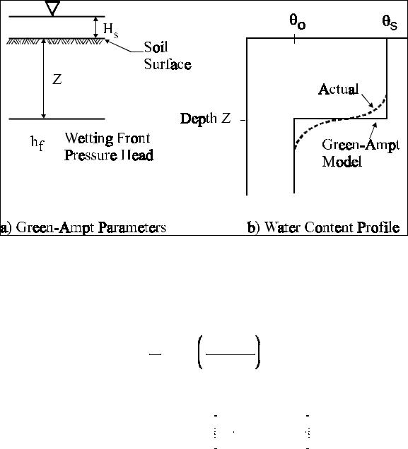
Green and Ampt assumed a piston-type water content profile (Figure 3) with a well-defined wetting front. The piston-type profile assumes the soil is saturated at a volumetric water content of s (except for entrapped air) down to the wetting front. At the wetting front, the water content drops abruptly to an antecedent value of 0, which is the initial water content. The soil-water pressure head at the wetting front is assumed to be hf (negative). Soil-water pressure at the surface, hs, is assumed to be equal to the depth of the ponded water.

Figure 3. Illustration of Green-Ampt parameters and the conceptualized water content profile, which demonstrates the sharp wetting front.

At any time, t, the penetration of the infiltrating wetting front will be Z. Darcy's law can be stated as follows:

where Ks is the hydraulic conductivity corresponding to the surface water content, and I(t) is the cumulative infiltration at time t, and is equal to Z( s- 0). Using this relation for I(t) to eliminate Z from Eq. 11, and performing the integration yields,

Equation 12 is precisely the statement of the Green-Ampt model. Philip (1957) demonstrated that the Green-Ampt equation can also be obtained as an exact solution of the Richards equation when the diffusivity function is assumed to be a Dirac Delta-type function with a non-zero value

7

only at the saturated water content. Philip called the Green-Ampt model the "delta-function" model.

4.2 Compilation of Green-Ampt Models

Even though originally developed for idealized conditions (i.e., homogeneous soil and constant surface ponding depth), the Green-Ampt model has been extended to take into account morerealistic features. Refer to Table 1 for a list of methods to estimate water flux based on the Green-Ampt model. Also, Appendix A is provided as an annotated bibliography pertaining to the Green-Ampt approach. The primary utility of the Green-Ampt approach lies in the estimation of the water flux, and it must be emphasized that the actual water content distribution with depth, (z), cannot be simulated, since the model formulation assumes a sharp wetting front.

Table 1. Models of Soil Water Movement Based on the Green-Ampt Concept1

1 Equation numbers referenced in this table correspond to those in the cited article. They do not correspond to the equation numbers in this report.

8

4.3 Parameter Estimation for the Green-Ampt Models

The popularity of the Green-Ampt models is primarily due to simplicity, adaptability to varying scenarios, and the availability of characteristic parameter values for various soil textures and conditions. Extensive studies conducted by the USDA's Agricultural Research Service (ARS) have resulted in the development of empirical relations for the model parameters in terms of easily-measurable variables. This has provided an additional impetus for the inclusion of GreenAmpt models in many watershed models (Goldman, 1989).

Bouwer (1966) demonstrated that Ks in Eq. 12 is not equal to the saturated hydraulic conductivity

of the soil (Ksat), but can be approximated as 0.5*Ksat. He also suggested that hf can be treated as air-exit suction head. Neuman (1976) derived expressions for hf, valid for small, intermediate,

and large times. Useful empirical expressions and various statistical correlations are available for Ks and hf (Brakensiek and Onstad, 1977; McCuen et al., 1981; Rawls and Brakensiek, 1982). Appendix C is provided to include additional references pertaining to the estimation of soil hydraulic parameters.

9