

Dressel.Gruner.Electrodynamics of Solids.2003
.pdf
|
|
6.4 |
Indirect and forbidden transitions |
159 |
||
for hω > Eg, and for the real part of the dielectric constant we obtain |
|
|||||
¯ |
|
|
|
|
1/2 |
|
|
e2 |
2µ |
|
|
||
|
|
|
|
|||
1(ω) = 1 + |
|
|
|
|
|pcv|2 |
|
m2ω2 |
h2 |
|
||||
|
|
¯ |
|
|
|
|
× 2Eg−1/2 − (Eg + h¯ ω)−1/2 − (Eg − h¯ ω)−1/2 {Eg − h¯ ω} |
(6.3.17) |
|||||
for frequencies near the gap energy; these frequency dependences are displayed in Fig. 6.9. In plotting these frequency dependences, it can be assumed that the matrix element |pcv| is constant, i.e. independent of frequency – by no means an obvious assumption.
6.4 Indirect and forbidden transitions
The results obtained above are the consequence of particular features of the dispersion relations and of the transition rate – the two factors which determine the optical transition. We have assumed that the maximum in the valence band coincides – in the reduced zone scheme – with the minimum in the conduction band, and we have also assumed that the first term in Eq. (6.2.10), the term ul (k)A · ul (k), is finite. In fact, either of these assumptions may break down, leading to interband transitions with features different from those derived above.
6.4.1 Indirect transitions
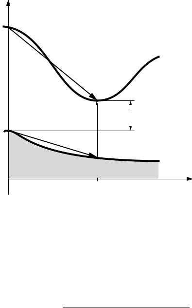
In a large number of semiconductors, the energy maxima in the valence and minima in the conduction bands do not occur for the same momentum k and k , but for different momenta; a situation sketched in Fig. 6.8b. Optical direct transitions between these states cannot take place due to momentum conservation; however, such transitions become possible when the excitation of phonons is involved. The two ways in which such so-called indirect transitions can occur are indicated in Fig. 6.11. One scenario involves the creation of a photon for wavevector k and the subsequent phonon emission, which absorbs the energy and momentum, necessary to reach the conduction band at momentum k . An opposite process, in which a phonon-involved transition leads to a valence state at k , followed by a photoninvolved vertical transition also contributes to the absorption process. In the two cases energy and momentum conservation requires that
Eg ± EP = h¯ ω
kl − kl = ±P ,
where P is the phonon momentum, and EP is the energy of the phonon involved. As before, it is understood that we use the reduced zone scheme, with all of its
160 |
6 Semiconductors |
P |
l' |
Energy E
Eg
P
l
k |
k' |
|
Wavevector k |
Fig. 6.11. Indirect transitions between the valence and conduction band states with different wavevectors. The dashed lines indicate the (vertical) transitions due to the interaction with photons, and the full straight lines indicate the transitions involving phonons with momenta P = k − k with energy EP. For both transitions Eg ± EP = h¯ ω, the energy of the vertical transition.
implications. We can use second order perturbation theory for the transition rate to obtain
W |
|
|
|
π e2 |
|
|
k |
|
q, l |
Vq (P, r) |
kl NP1/2 kl |A · Pl l |kl |
|
2 |
||||||||||||
|
(k,l)→(k+P,l ) = |
|
|
|
|
|
|
+ |
|
|
| |
|
|
kl |
| |
|
|
kl |
hω |
|
|
||||
|
2m2hc2 |
|
|
|
|
|
|
|
|
E |
− E |
|
|
||||||||||||
|
|
|
|
|
¯ |
|
|
|
|
|
|
|
|
|
|
|
|
− ¯ |
|
|
|
||||
|
|
|
|
|
|
|
|
|
|
|
|
|
|
|
|
|
|
|
|
|
|
|
|
|
|
|
|
× |
δ |
k |
P,l |
− E |
kl |
− |
hω |
|
hωP |
} |
|
, |
(6.4.1) |
||||||||||
|
|
|
{E + |
|
|
|
|
¯ |
− ¯ |
|
|
|
|
|
|
|
|||||||||
where NP denotes the phonon occupation number, and ωP is the frequency of the phonons involved. This in thermal equilibrium is given by the Bose–Einstein
6.4 Indirect and forbidden transitions |
161 |
||||||
expression |
|
|
|
|
|
|
|
NP |
|
|
1 |
|
. |
(6.4.2) |
|
|
|
|
|
|
|||
= exp |
k¯BT |
|
|||||
|
− 1 |
|
|||||
|
|
|
|
hωP |
|
|
|
In Eq. (6.4.1) the first angled bracket involves the transition associated with the phonons, and the second involves the vertical transition. Similar expressions hold for other transitions indicated in Fig. 6.11.
The matrix elements are usually assumed to be independent of the k states involved, and the transitions may occur from valence states with different momenta to the corresponding conduction states, again with different momentum states. Therefore we can simply sum up the contributions over the momenta k and k in the delta function. Converting the summation to an integral as before, we obtain
Wllind(ω) NP Dl (El )Dl (El )δ{El − El − h¯ ω ± h¯ ωP} dEl dEl . (6.4.3)
The two transitions indicated in Fig. 6.11 involve different phonons, and also different electron states in the valence and conduction bands. Unlike the case of direct vertical transitions, there is no restriction to the momenta k and k , as different phonons can absorb the momentum and energy required to make the transition possible. Consequently, the product Dl (El ) · Dl (El ) – instead of the joint density of states Dl l (E) – appears in the integral describing the transition rate. This then leads to an energy dependence for the indirect optical transition which is different from the square root behavior we have found for the vertical transition (Eq. (6.3.11)), and calculations along these lines performed for the direct transition lead to
2 |
(ω) NP(Eg − EP ± hω)2 |
(6.4.4) |
|
¯ |
|
for h¯ ω ≥ Eg ± EP.
Such indirect transitions have several distinct characteristics when compared with direct transitions. First, the absorption coefficient increases with frequency as the square of the energy difference, in contrast to the square root dependence found for direct transitions. Second, the absorption is strongly temperature dependent, reflecting the phonon population factor NP; and third, because of the two processes for which the phonon energy appears in different combinations with the electronic energies, two onsets for absorption appearing at different frequencies are expected. All these make the distinction between direct and indirect optical transitions relatively straightforward.
162 |
6 Semiconductors |
6.4.2 Forbidden transitions
Let us now return to Eq. (6.2.10), which describes the transition between two bands. The first integral on the right hand side
ieh 1 |
|
l |
· |
|
|
||
2mc |
|
||||||
¯ |
|
|
|
u (k)[A |
|
ul |
(k)] dr |
is involved in the direct transitions we discussed in Section 6.2.2. For a perfect semiconductor, for which all states in the valence and conduction bands can be described by Bloch functions, the second part of the Hamiltonian, i.e. the matrix element
ieh 1 |
|
l |
· |
|
|
|||
2mc |
|
|||||||
¯ |
|
|
|
|
u (k) [iA |
|
k ul |
(k)] dr , |
would be identical to zero simply because the wavefunctions are orthogonal in the different bands. Small changes in k (due to phonons or other scatterers) may, however, violate this strict rule and lead to a finite integral – and thus contribute to the optical transitions between the valence and conduction bands. Of course, the integral remains small compared to the integral which describes the direct transitions, and can be of importance only when the direct allowed transitions do not occur – due to the vanishingly small matrix element involved in these transitions. Let us assume that due to these scattering processes transitions between (slightly) different k states are possible, and expand the product for small wavevector differences k = k − k :
|
ul (k )ul (k) dr ≈ |
ul (k ) 1 + k · k + |
1 |
(k · k)2 + · · · ul (k) dr . |
|
||||
2 |
(6.4.5) The first term in the integral is zero; the second term is also zero if the allowed transition has a zero matrix element (see the first term in Eq. (6.2.10)) – as should be the case when forbidden transitions make the important contribution to the absorption; and the third term is proportional to (k )2 and is therefore small. Thus, as a rule, forbidden transitions have significantly smaller matrix elements than direct transitions.
Calculation of the optical absorption for such higher order transitions proceeds along the lines we have followed before. The term introduces extra k2 factors, and thus additional energy dependences; we find upon integration that
2(ω) h¯ ω − Eg |
3/2 , |
(6.4.6) |
a functional form distinctively different from that which governs the direct absorption.
6.5 Excitons and impurity states |
163 |
6.5 Excitons and impurity states
Finally we discuss optical transitions in which states brought about by Coulomb interactions are of importance. Electron–hole interactions lead to mobile states, called excitons, whereas Coulomb interactions between an impurity potential and electrons lead to bound states localized to the impurity sites. In both cases, these states can be described simply, by borrowing concepts developed for the energy levels of single atoms.
6.5.1 Excitons
When discussing the various optical transitions, we used the simple one-electron model, and have neglected the interaction between the electron in the conduction band and the hole remaining in the valence band. Coulomb interaction between these oppositely charged entities may lead to a bound state in a semiconductor, and such bound electron–hole pairs are called excitons. Such states will have an energy below the bottom of the conduction band, in the gap region of the semiconductor or insulator. As the net charge of the pair is zero, excitons obviously do not contribute to the dc conduction, but can be excited by an applied electromagnetic field, and will thus contribute to the optical absorption process.
For an isotropic semiconductor, the problem is much like the hydrogen atom problem, with the Coulomb interaction between the hole and the electron screened by the background dielectric constant 1 of the semiconductor. Both hole and electron can be represented by spherical wavefunctions, and the energy of the bound state is given by the usual Rydberg series,
Eexcj |
= Eg − |
e4µ |
(6.5.1) |
||
|
|
, |
|||
2h2 |
2 j2 |
||||
|
|
¯ |
1 |
|
|
where j = 1, 2, 3, . . . and µ−1 = mv−1 + mc−1 denotes the effective mass we have encountered before. The low frequency dielectric constant is 1 = 1+C h¯ ωp/Eg 2 with C a numerical constant of the order of one, as in Eq. (6.3.6). The spatial extension of this state can be estimated by the analogy to the hydrogen atom, and we find that
rexc |
|
|
h2 j2 |
||
= |
1 |
¯ |
. |
||
j |
e2 |
µ |
|
||
For small bandgap semiconductors, the static dielectric constant 1 is large, and consequently the spatial extension of the excitons is also large. At the same time, according to Eq. (6.5.1), the energy of the excitons is small. This type of electron– hole bound state is called the Mott exciton and is distinguished from the strongly
6.5 Excitons and impurity states |
165 |
Here we are interested in the optical signature of these exciton states. Instead of free electrons and holes – the energy of creating these is the gap energy Eg or larger – the final state now corresponds to the (ideally) well defined, sharp, atomic like energy levels. Transitions to these levels then may lead to a series of well defined absorption peaks, each corresponding to the different j values in the Rydberg series. The energy separation between these levels is appreciable only if screening is weak, and this happens for semiconductors with large energy gaps. For small bandgap semiconductors, the different energy levels merge into a continuum, especially with increasing quantum numbers j. Transitions to this continuum of states – with energy close to Eg – lead to absorption near the gap, in addition to the absorption due to the creation of a hole in the valence band and an electron in the conduction band. The calculation of the transition probabilities is a complicated problem, beyond the scope of this book.
6.5.2 Impurity states in semiconductors
Impurity states, created by acceptor or donor impurities, and the extrinsic conductivity associated with these states (together with the properties of semiconductor junctions) have found an enormous number of applications in the semiconductor industry. Of interest to us are the different types of energy levels – often broadened into a band – which these impurity states lead to in the region of the energy gap. Various optical transitions between these energy levels and the conduction or valence bands are found, together with transitions between these impurity levels.
The impurity states are usually described in the following way. One atom in the crystal is replaced by an atom with a different charge – say a boron atom in a silicon crystal. It is regarded as an excess negative charge at the site of the doping and a positive charge loosely bound to this position (loosely because of the screening by the electrons in the underlying semiconductor). The model which can account for this, at least for an isotropic medium, is Bohr’s model of an atom, and the energy levels are
Eimpj |
= |
e4m |
(6.5.3) |
|
2h2 |
2 j2 |
|||
|
|
¯ |
1 |
|
where j = 1, 2, 3, . . . , m is the effective mass of electrons or holes, and 1 is the background dielectric constant; here the energy is counted from the top of the valence band. There is a mirror image of this in the case of doping with a donor; the energy levels as given by the above equation are then negative in sign, and are measured from the bottom of the conduction band. These states are shown in a schematic way in Fig. 6.13. The energy scales associated with impurity states are
6.5 Excitons and impurity states |
167 |
increases strongly with increasing temperature. The various aspects of this socalled extrinsic conduction mechanism are well known and understood.
Electron states can also be delocalized by increasing the impurity concentration, and – because of the large spatial extension of the impurity states – the overlap of impurity wavefunctions, and thus delocalization occurs at low impurity concentrations. Such delocalization leads to a metallic impurity band, and this is a prototype example of (zero temperature) insulator-to-metal transition.
All this has important consequences on the optical properties of doped semiconductors. For small impurity concentrations, transitions from the valence band to the impurity levels, or from these levels to the continuum of states, are possible, leading to sharp absorption lines, corresponding to expression (6.5.3), together with transitions between states, corresponding to the different quantum numbers j. Again, the transition states between the continuum and impurity states are difficult to evaluate; but transitions between the impurity levels can be treated along the lines which have been developed to treat transitions between atomic energy levels. Interactions between impurities at finite temperatures all lead to broadening of the (initially sharp) optical absorption lines.
The situation is different when impurity states are from a delocalized, albeit narrow, band. Then what is used to account for the optical properties is the familiar Drude model, and we write
σ1(ω) = |
N j e2τ |
|
1 |
(6.5.4) |
1m j |
1 + ω2τ 2 |
|||
where N j is the number of impurity states, m j is the mass of the impurity state, and τ is the relaxation time; 1 is again the background dielectric constant. This then leads to the so-called free-electron absorption together with a plasma edge at
ωp = |
4 |
π N e2 |
|
1/2 |
≈ |
N m |
|
1/2 |
|
j |
|
j |
Eg . |
(6.5.5) |
|||||
|
1m j |
|
N m j |
As m ≈ m j and N j N , the plasma edge lies well in the gap region and is also dependent on the dopant concentration. The optical conductivity and reflectivity expected for a doped semiconductor (in the regime where the impurities form a band, and the impurity conductivity is finite at zero frequency) are displayed in Fig. 6.14; the parameters chosen are appropriate for a dc conductivity σdc = 2 × 10⁴ −1 cm−1 and a scattering rate 1/(2π τ c) = 0.2 cm−1; the energy gap between the conduction and valence bands is νg = Eg/ hc = 1000 cm−1.