Dressel.Gruner.Electrodynamics of Solids.2003

in the frequency domain. Whereas scalar network analyzers evaluate only the magnitude of the signal, vector network analyzers deliver magnitude and phase, i.e. the complex impedance, or alternatively the so-called scattering matrix or transfer function.

The sample is usually placed between the two conductors of a coaxial line or the walls of a waveguide. Calibration measurements are required to take effects into account, for example the resistance, stray capacitance, and inductance of the leads. For special requirements – concerning the accuracy, output power, or stability – monochromatic solid state sources (such as Gunn diodes or IMPATT sources) are utilized as generators in custom made setups instead of network analyzers.

Optical measurements

If the wavelength λ is much smaller than the sample size a, the considerations of geometrical optics apply and diffraction and boundary effects become less important; by rule of thumb, diffraction and edge effects can be neglected for a > 5λ. In contrast to lower frequencies, phase information cannot be obtained. Standard power reflection measurements are performed in an extremely wide frequency range, from millimeter waves up to the ultraviolet (between 1 cm−1 and 106 cm−1); they are probably the single most important technique of studying the electrodynamic properties of solids.

Although tunable, monochromatic radiation sources (such as backward wave oscillators, infrared gas lasers, solid state and dye lasers) are available in the infrared, visible, and ultraviolet frequency range, it is more common that broadband sources are used and dispersive spectrometers (grating and prism spectrometers) are employed to select the required frequency. For the latter case, either a certain frequency of the radiation is selected (either by dispersing prisms or by utilizing diffraction gratings) which is then guided to the specimen, or the sample is irradiated by a broad spectrum but only the response of a certain frequency is analyzed. Combined with suitable detectors the relative amount of radiation at each frequency is then recorded.

Because of their great light efficiency, single order spectrum, ruggedness, and ease of manufacture, prisms have long been favored as a dispersing medium in spectrographs and monochromators in the visible spectral range. The disadvantages of prisms are their non-linear dispersion and the limited frequency range for which they are transparent. If high resolution is required, grating spectrometers are commonly used as research instruments. Two or more monochromators may be employed in series to achieve higher dispersion or greater spectral purity; stray light is also greatly reduced [Dav70].

Optical experiments are in general performed in a straightforward manner by measuring, at different frequencies, either the bulk reflectivity or both the trans-

mission and reflectivity. If the investigations are conducted on samples of different thickness, the real and imaginary parts of the response can be evaluated. Measurements of the complex optical properties are also possible using Mach–Zehnder interferometers or Fabry–Perot resonators as discussed in Section 11.3.4.

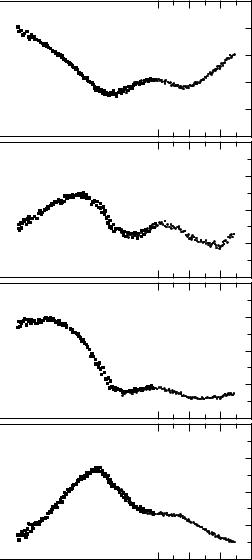
As an example of an optical experiment performed in the frequency domain, data from a room-temperature transmission experiment on TlGaSe2 are displayed in Fig. 10.1. Fig. 10.1a shows the frequency dependence of the power transmission TF through a 1 mm slab of TlGaSe2; the corresponding phase shift φt – as obtained by a Mach–Zehnder interferometer using a coherent radiation source (Section 11.2.3) – is plotted in Fig. 10.1b. Following the analysis laid out in Section 2.4.2, for each frequency point these two parameters TF and φt allow evaluation of both components of the complex dielectric constant ˆ = 1 + i 2 as shown in Fig. 10.1c,d. There a strong absorption peak centered at 14 cm−1 and a shoulder around 19 cm−1; the maximum of 2 corresponds to a minimum of transmission. The phase shift is mainly determined by the real part of the dielectric constant. A peak in 2(ω) leads to a step in 1(ω) as we have already seen in the simple model of a Lorentzian oscillator (Fig. 6.3).

10.2 Time domain spectroscopy

Instead of measuring the response of a solid by applying monochromatic radiation varied over a wide frequency range, the optical constants can also be obtained by performing the experiment in the time domain using a voltage pulse with a very short rising time. Such a pulse – via the Laplace transformation presented in Appendix A.2 – contains all the frequencies of interest. In general, a linear time invariant system can be described unequivocally by its response to an applied pulse. Two basic setups are employed depending on the frequency range of importance: either the sample is placed in a capacitor and the charging or discharging current is observed; or a voltage pulse is applied at a transmission line and the attenuation and broadening of the pulse upon passing through the sample placed in this line is observed. The latter method can also be used in free space by utilizing an optical setup. In both cases, from this information 1 and σ1 of the material can be determined by utilizing the Laplace transformation. Crudely speaking, the losses of the material cause the attenuation of the pulse while the real part of the dielectric constant is responsible for the broadening.

The experimental problem lies in the generation and detection of suitable pulses or voltage steps. Short pulses of electromagnetic radiation are generated by fast switches or by electro-optical configurations. Although with a voltage step of rise time t the entire spectrum up to approximately 1/t can be covered, time domain

experiments are preferably performed in those parts of the spectrum where no standard techniques are available in the frequency domain.

10.2.1 Analysis

The objective of time domain spectroscopy is to evaluate the complex response function χˆ (ω) by analyzing the time dependent response P(t). To this end the mathematical methods of the Laplace transformation are used as described in Appendix A.2. In a linear and causal system, the general response P(t) to a perturbation E(t) can be expressed by

where χ (t) is the response function in question. Note that χ is not local in time, meaning that P(t) depends on the responses to the perturbation E(t) for all times t prior to t. The equation describes a convolution P(t) = (χ E)(t) as defined in Eq. (A.2b), leading to the Fourier transform:

Thus for a known time dependence of the perturbation E(t) we can measure the response as a function of time P(t) and immediately obtain the frequency dependent response function χ (ω):

If the system is excited by a Dirac delta function E(t) = δ(t), the response directly yields χ (t). Then the convolution simplifies to P(t) = (χ δ)(t) = χ (t), and the frequency dependence is the Fourier transform of the pulse response given by

which can also be obtained from Eq. (10.2.3) with the help of Eq. (A.1): E(ω) = 1. Another commonly used perturbation is a step function

where we have to replace the Fourier transform by the Laplace transform in order

10.2.2 Methods

Time domain spectroscopy is mainly used in frequency ranges where other techniques discussed in this chapter – frequency domain spectroscopy and Fourier transform spectroscopy – have significant disadvantages. At very low frequencies (microhertz and millihertz range), for instance, it is not feasible to measure a full cycle of a sinusoidal current necessary for the frequency domain experiment. Hence time domain experiments are typically conducted to cover the range from 10−6 Hz up to 106 Hz. Of course, also in the time domain, data have to be acquired for a long period of time to obtain information on the low frequency side since both are connected by the Fourier transformation, but the extrapolation for t → ∞ with an exponential decay, for example, is easier and often well sustained.

As we have seen in Section 8.3, from 10 GHz up to the terahertz range, tunable and powerful radiation sources which allow experiments in the frequency domain are not readily available. Even for the use of Fourier transform techniques, broadband sources with sufficient power below infrared frequencies are scarce. To utilize time domain spectroscopy in this range requires extremely short pulses with an inverse rise time comparable to the frequency of interest. Due to recent advances in electronics, pulses of less than one nanosecond are possible; using short pulse lasers, pulses with a rise time of femtoseconds are generated. In these spectral ranges time domain methods are well established.

We consider three cases, employed in three different ranges of the electromagnetic spectrum. First, the sample is placed in a capacitor and the characteristic discharge is determined; this is a suitable setup for experiments on dielectrics at the lower frequency end of the spectrum. In a second arrangement, a short electrical pulse travels along a coaxial cable or waveguide which contains the sample at one point; the change in intensity and shape of the pulse due to reflection off or transmission through the sample is measured. The third setup utilizes a similar principle, but is an optical arrangement with light pulses of only a few picoseconds duration traveling in free space; here the transmission and time delay are probed.

Audio frequency time domain spectroscopy

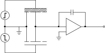
Time domain spectroscopy is useful for studying slow processes in the frequency range down to microhertz, where the frequency domain method faces inherent limits such as stability or long measurement times [Hil69, Hyd70, Sug72]. To determine the complex dielectric constant, a voltage or current step is applied and the time decay of the charging or discharging current or voltage, respectively, is monitored. Fig. 10.2 shows the basic measurement circuit which can be used to investigate low-loss samples at very low frequencies. Voltage steps of equal magnitude but opposite polarity are applied simultaneously to the two terminal capacitors Cx and Cr. Cr is an air filled reference capacitor, and Cx contains the specimen

254 10 Spectroscopic principles

Fig. 10.2. Measurement circuit of a dielectric spectrometer for time domain investigations in the low frequency range. The generators G+ and G− apply positive and negative voltage steps across the sample capacitor Cx and the reference capacitor Cr, respectively. The charge detector, formed by the operational amplifier and feedback capacitor Cf, provides an output proportional to the net charge introduced by the step voltage.

of the material to be studied. The symmetric design compensates the switching spike and hence considerably reduces the dynamic-range requirements. For better conducting samples the influence of the contacts becomes more pronounced and the discharge is faster.

In the special case of a step voltage, dPstep(t)/dt is related to the charging current density by Eq. (10.2.5b), and finally we find for the real and imaginary parts of the

dielectric constant of the sample

One assumption of this analysis is the linearity and causality of the response. Due to the fact that the Kramers–Kronig relations are inherently utilized, both components of the dielectric response are obtained by the measurement of only one parameter. Equally spaced sampling presents an experimental compromise between the resolution needed near the beginning of the detected signal and the total sampling time necessary to capture the entire response. As mentioned above, the short spacing at the start is needed for the high frequency resolution, and the long-time tail dominates the low frequency response. Non-uniform sampling, i.e. stepping the intervals logarithmically, however, precludes the applicability of well developed algorithms, such as the fast Fourier transformation.

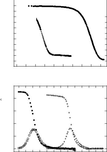
As an example, the time dependent polarization P(t) of propylene carbonate after switching off the applied electric field is displayed in Fig. 10.3a. Applying

Polarization P

Propylene carbonate

Fig. 10.3. (a) Time dependent polarization P(t) of propylene carbonate at two temperatures T = 155 K and 166 K measured after switching the electric field off. (b) Real and imaginary parts of the frequency dependent dielectric constant ˆ( f ) obtained by Laplace transformation of the time response shown in (a) (after [Boh95]).

Eqs (10.2.8), the frequency dependent dielectric constant is calculated and plotted in Fig. 10.3b. The data were taken from [Boh95]. The dielectric relaxation strongly depends on the temperature, and the time dependence deviates from a simple exponential behavior. The slow response at low temperatures (155 K) corresponds to a low frequency relaxation process.

Radio frequency time domain spectroscopy

The time dependence of a voltage step or pulse which travels in a waveguide or a coaxial cable line, and is reflected at the interface between air and a dielectric medium, can be used to determine the high frequency dielectric properties of the material. From the ratio of the two Fourier transforms, the incident and the reflected signals, the scattering coefficient is obtained; and eventually the complex response spectrum of the sample can be evaluated using the appropriate expressions derived in Section 9.2. Similar considerations hold for a pulse being transmitted through a sample of finite thickness. Fast response techniques permit measurements ranging from a time resolution of less than 100 ps, corresponding to a frequency range up to 10 GHz.

A time domain reflectometer consists of a pulse generator, which produces a voltage step with a rise time as fast as 10 ps, and a sampling detector, which transforms the high frequency signal into a dc output. The pulse from the step generator travels along the coaxial line until it reaches a point where the initial voltage step is detected for reference purposes; the main signal travels on. At the interface of the transmission line and the sample, part of the step pulse will be reflected and then recorded. Comparing both pulses allows calculation of the response function of the sample. The time dependent response to a step function perturbation is widely used for measurements of the dielectric properties, mainly in liquids, biological materials, and solutions where long-time relaxation processes are studied. A detailed discussion of the different methods and their analysis together with their advantages and disadvantages can be found in [Fel79, Gem73].

Terahertz time domain spectroscopy

In order to expand the time domain spectroscopy to higher frequencies in the upper gigahertz and lower terahertz range, two major changes have to be made. Due to the high frequencies, guided transmission by wires or waveguides is not feasible and a quasi-optical setup is used. Furthermore, the short switching time required is beyond the capability of an electronic device, thus short optical pulses of a few femtoseconds furnished by lasers are utilized. Here the sudden discharge between two electrodes forms a transient electric dipole and generates a short electromagnetic wave which contains a broad range of frequencies; its center frequency corresponds to the inverse of the transient time. Terahertz spectroscopy measures two electromagnetic pulse shapes: the input (or reference) pulse and the propagated pulse which has changed shape owing to its passage through the sample under study. We follow the discussion of Section 10.2.1, but as the response function χˆ (ω) we now use the complex refractive index Nˆ (ω), which describes the wave propagation, or the conductivity σˆ (ω), which relates the current density to

I

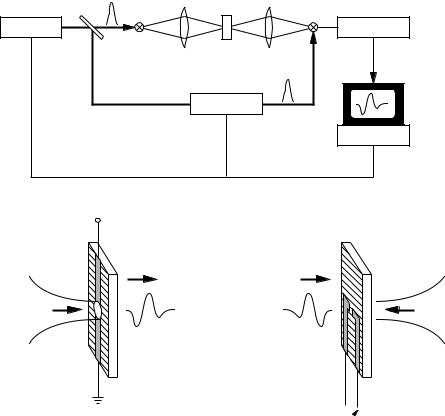
Fig. 10.4. (a) Schematic of a terahertz (THz) time domain spectrometer. The femtosecond laser pulse drives the optically gated THz transmitter and – via beamsplitter and delay line

– the detector. The THz radiation is collimated at the sample by an optical arrangement.

(b) The radiation source is an ultrafast dipole antenna which consists of a charged transmission line. The beam spot of the femtosecond pulses is focused onto the gap in the transmission line and injects carriers into the semiconductor leading to a transient current flowing across the gap, which serves as a transient electric dipole. (c) In order to detect the THz radiation, a similar arrangement is used. The current flows though the switch only when both the THz radiation and photocarriers created by the femtosecond laser beam are present.

the electric field applied. Equation (10.2.1) then reads:

J(t) = σˆ (t − t )E(t ) dt .

A terahertz time domain spectrometer is displayed diagrammatically in